Determining Redshifts
Updated: Aug25,2020 Primary List

Introduction.

Here we cover some routines used to measure galaxy redshifts from spectra. Some of the sections below will deal with setting up and recieving reduced HET spectra, but our primary concern is this: with a digital galaxy spectrum, how do we identify specralfeatures and use them to compute the radial velocity of the galaxy? I have three routines that are useful for this, and you can read online documentation for each with this commands:

 
% speclines.sh --help     # Make a list of spectral features  
% redshift.sh --help      # Given identified spectral features, compute a mean redshitf 
% redshifter.sh --help    # Given a redshift, predict observed wavelengths

These routines are used to identify specrtal features with known restframe wavelenths in a specturm and compute a corresponding radial velocity. The routine speclines.sh enables us to select line lists from a library of spectral features. The library started out including just a few common features for early- and late-type galaxies. It has grown, but basically still enables the user to access the rest-frame wavelengths and text-style names for spectral lines

The redshift.sh and redshifter.sh are inverse routines. The first will compute a radial given a set of identified spectral features, the second will predict a the observed wavelengths for a set of spectral features given a radial velocity. To help identify features viaually, I have a developed spec_selector (a modified version of the code point_selector ).

I have prepared a simple example of determining a redshift based on the spectrum present below that S.Janowieki and I observed for Jimi Lowrye in May 2020. In this simple example I cover how I use the routines above to compute a redshift given our digital spectrum from LRS2.

Return to top of page.

Setting up HET observations with TSL.

A lot of the spectrum analysis I do uses HET observations. I have compiled a short set of notes and figures on setting up HET observations with TSL.

Return to top of page.

An LRS2-B observation of 1Zw136

Here is a Jimi L observation.

 
% redshitf.sh --help

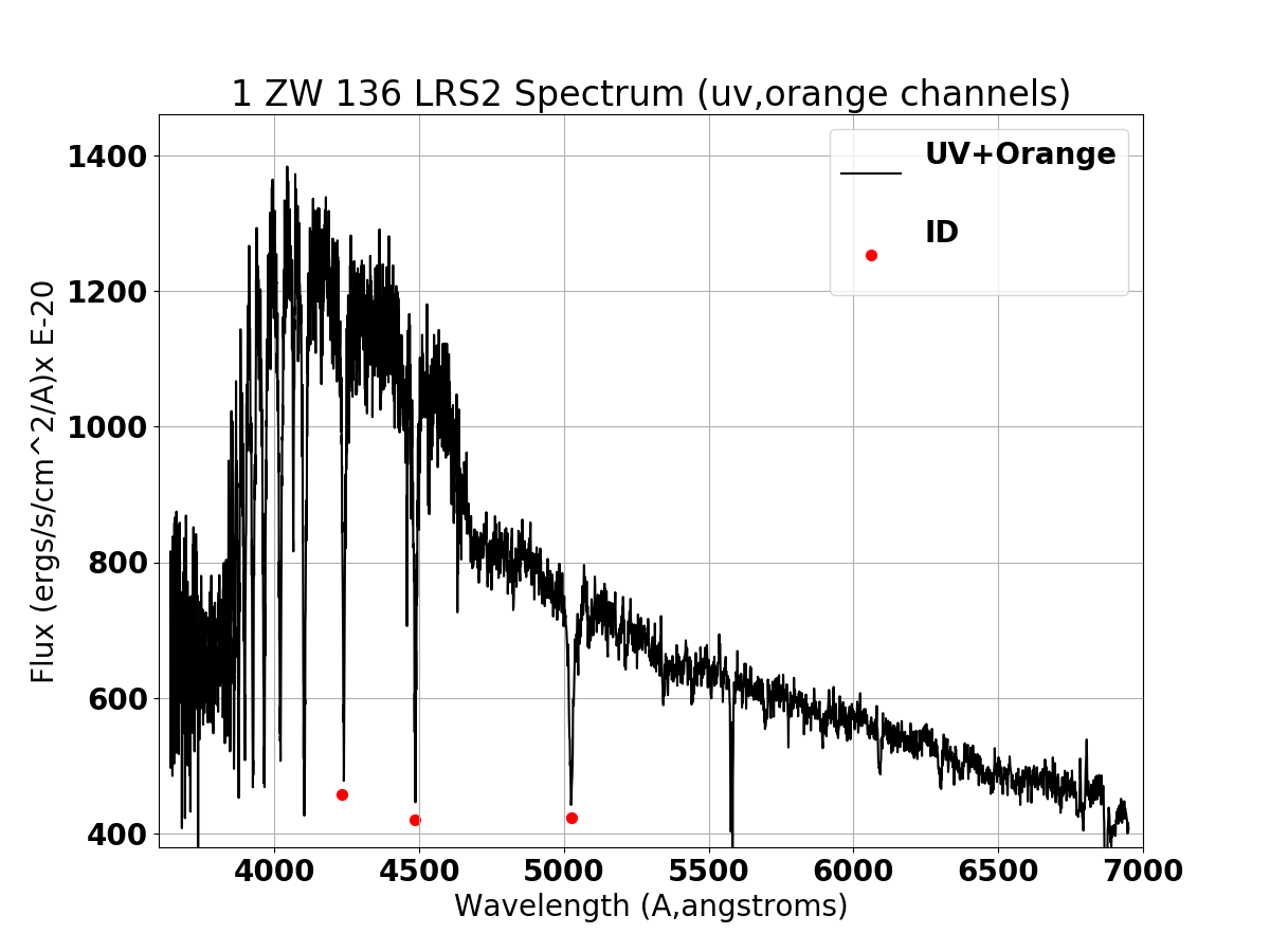A 1-D spectrum from UV and Orange channels of a 20200529 LRS2-B spectrum of 1 ZW 136 (Ra,Dec = 16:13:30.19 +51:03:35.6) is shown. I have identified 3 lines that are marked by the red circles: from right to left thay are H_beta, H_gamma, and H_delta. The continuum for this specturm appears to be much to vlue for an ordinary E+A galaxy, but I simply wanted to see how close these identifications, made manually with an interactive plotting routine, might agrree. The results are summarized below:


   Wave_obs     Wave_rest      Feautre            Vobs(km/s)
    4238.900      4101.740     H_delta             10031.8
    4486.300      4340.470     H_gamma             10079.3
    5025.100      4861.330     H_beta_L            10106.5
    Mean Velocity =    10072.534  -+  21.822  km/s

The mean error of ±21.8 km/s is surprisingly small.

Later I refined the LRS2 spectrum plotting process and I now have the results below.

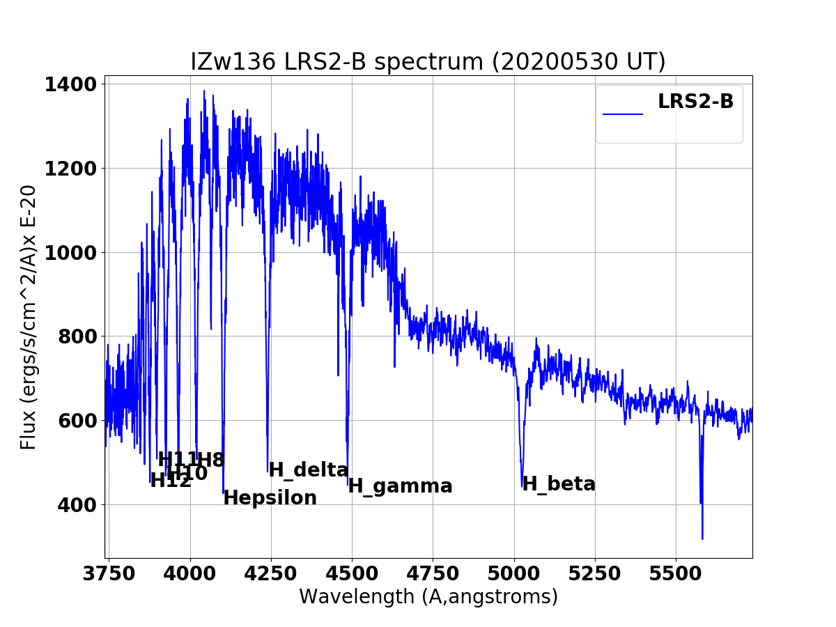A 1-D spectrum from UV and Orange channels of a 20200529 LRS2-B spectrum of 1 ZW 136 (Ra,Dec = 16:13:30.19 +51:03:35.6) is shown. I have identified 8 Balmer absorption lines that are labeled above. The continuum for this specturm appears to be much bluer than for an ordinary E+A galaxy, but the feature identifications seem secure. Rejecting the H_epsilon line, the final table of radial velocity values is shown below


  Wave_rest   Feautre    Wave_obs    V(km/s)     
   4101.74    H_delta    4239.69    10082.46    
   4340.47    H_gamma    4484.69     9960.98    
   4861.33    H_beta     5023.62    10008.04    
   3750.15    H12        3875.03     9982.75    
   3770.63    H11        3897.95    10122.78    
   3797.90    H10        3924.75    10012.76    
   3889.05    H8         4018.96    10014.48    
   Mean Velocity =    10026.3 ± 21.5 km/s
   mean redshift, z =  0.0334 ± 0.0001

In Aug2020 I spent some time studying up on numpy (see NumPy Studies and in the course of that I developed gregz_002.py (a modified version of a simple GregZ code). I used this to analyza and play with the data cube from Greg that combines the ouv and orange channels into one data cube. I used this two make the two plots below.

 

See notes in /home/sco/jimiL/red_Aug25_2020/Aug25_01/README.red_Aug25_2020
Data cube = eng_galaxy_1_LRS2B_cube.fits
% python gregz_002.py

% cp spectrum.dat spectrum.dat_sco
% vi spectrum.dat_sco                       # just remove header stuff
% cubespec.sh spectrum.dat_sco
Flux min,max = -0.2713111E-15    0.4244979E-15
Enter desired exponent (-14): -19
4727 3 

Resulting file = spectrum.table  (and params,parlab files) 

% mkdir plot1
% cd plot1
% cp ../spectrum.table .
% cp ../spectrum.parlab .
% Generic_Points N
% getrc 
% xyplotter_auto spectrum wave flux 1 N
% xyplotter List.1 Axes.1 N

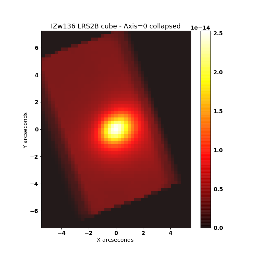
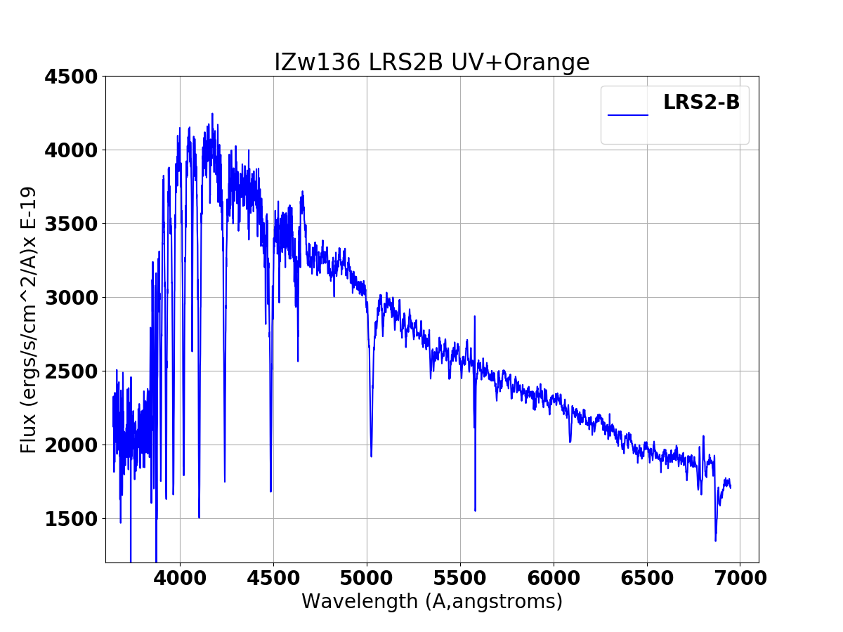
GregZ's data cibe (eng_galaxy_1_LRS2B_cube.fits) was collapsed with gregz_002.py to give an integrated light image covering signal from 3640 angstroms to 6949 angstroms.

IZw136 LRS2-B spectrum extracted with R=1.5 arcsecond circular aperture.

Return to top of page.

Back to calling page