1. Introduction.

In May of 2020 (the night of 20200530 UT) we obtained an LRS2-B observation of IZw136 for Jimi Lowrey. I used the public HET night report reader to collect this information about the observation:

 
HET night report reader: https://het.as.utexas.edu/HET/hetweb/vlrweb/RR/reader.php
NOTE:  Click the very top banner (HET Night Report Reader) to go to: 
https://het.as.utexas.edu/HET/hetweb/vlrweb/RR/index.php
From here you can navigate to any night in question. 

The night that Jimi's observations were made:    May29,2020   (2020-05-29)   Civil Date!!!!
Recall the NR sysetme uses civil dates, not UT. 

The observation for JL: 
LRS image             = lrs20000009_01 
target name           = eng_galaxy_1_056_E	
Exposure start time   = 04:21 UT 
Exposure (seconds)    = 600	
progran number        = ENG20-2-000

Also of interst:
 twilight flats                          =  lrs20000002_01 to lrs20000007_01
  BD+28_4211_056_E (LRS2-B spc standard) = lrs20000011_01      (9:48 UT) 
  BD+28_4211_056_E (LRS2-R spc standard) = lrs20000012_01      (9:51 UT) 

LRS2 cals = obs=20-25 (arcs and lamps), obs=1 (exp1-11) (bias)      

Originally I used pipeline reductions from GrgZ's panacea code that I retrieved form TACC :
ssh sodewahn@wrangler.tacc.utexas.edu    (_scotacc and token 2F)
To pull the cube files I used: 
% scp -r sodewahn@wrangler.tacc.utexas.edu:/work/03946/hetdex/maverick/LRS2/ENG20-2-000/20200530_0000009_exp01_\*_cube.fits .

--------------
For completeness, I am also pulling the raw lrs2 and acm /hetedata/data directories 
for that night (20200530 UT): 

[sco@mcs 20200530]$ pwd
/home/mcs/sco/HET_IZw136/20200530
[sco@mcs 20200530]$ cp -r /hetdata/data/20200530/lrs2 .
[sco@mcs 20200530]$ cp -r /hetdata/data/20200530/acm .

I transfer this directory to sco2019: 
% pwd
/home/sco/jimiL_IZw136
% scp -r sco@buckaroo.as.utexas.edu:/home/buckaroo/sco/HET_IZw136 .
**** NOTE: I also pulled 20200529 in case I want lrs2 cals from the early evening. 
% /home/sco/jimiL_IZw136/HET_IZw136

 
% redshitf.sh --help  
 

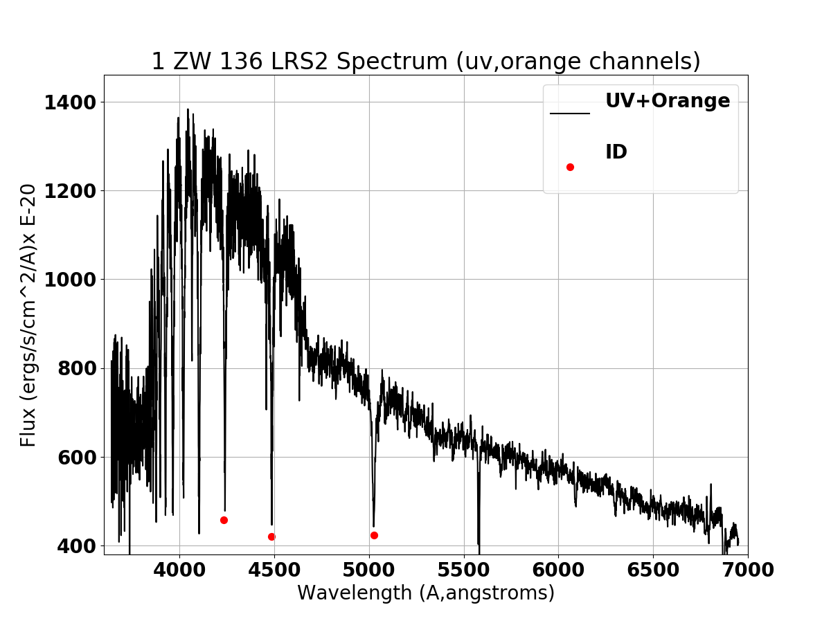A 1-D spectrum from UV and Orange channels of a 20200530 LRS2-B spectrum of 1 ZW 136 (Ra,Dec = 16:13:30.19 +51:03:35.6) is shown. I identified 3 lines that are marked by the red circles: from right to left thay are H_beta, H_gamma, and H_delta. The continuum for this specturm appears to be much to vlue for an ordinary E+A galaxy, but I simply wanted to see how close these identifications, made manually with an interactive plotting routine, might agrree. The results are summarized below: Wave_obs Wave_rest Feautre Vobs(km/s) 4238.900 4101.740 H_delta 10031.8 4486.300 4340.470 H_gamma 10079.3 5025.100 4861.330 H_beta_L 10106.5 Mean Velocity = 10072.534 -+ 21.822 km/s The mean error of ±21.8 km/s is surprisingly small.

Later I refined the LRS2 spectrum plotting process and I now have the results below.

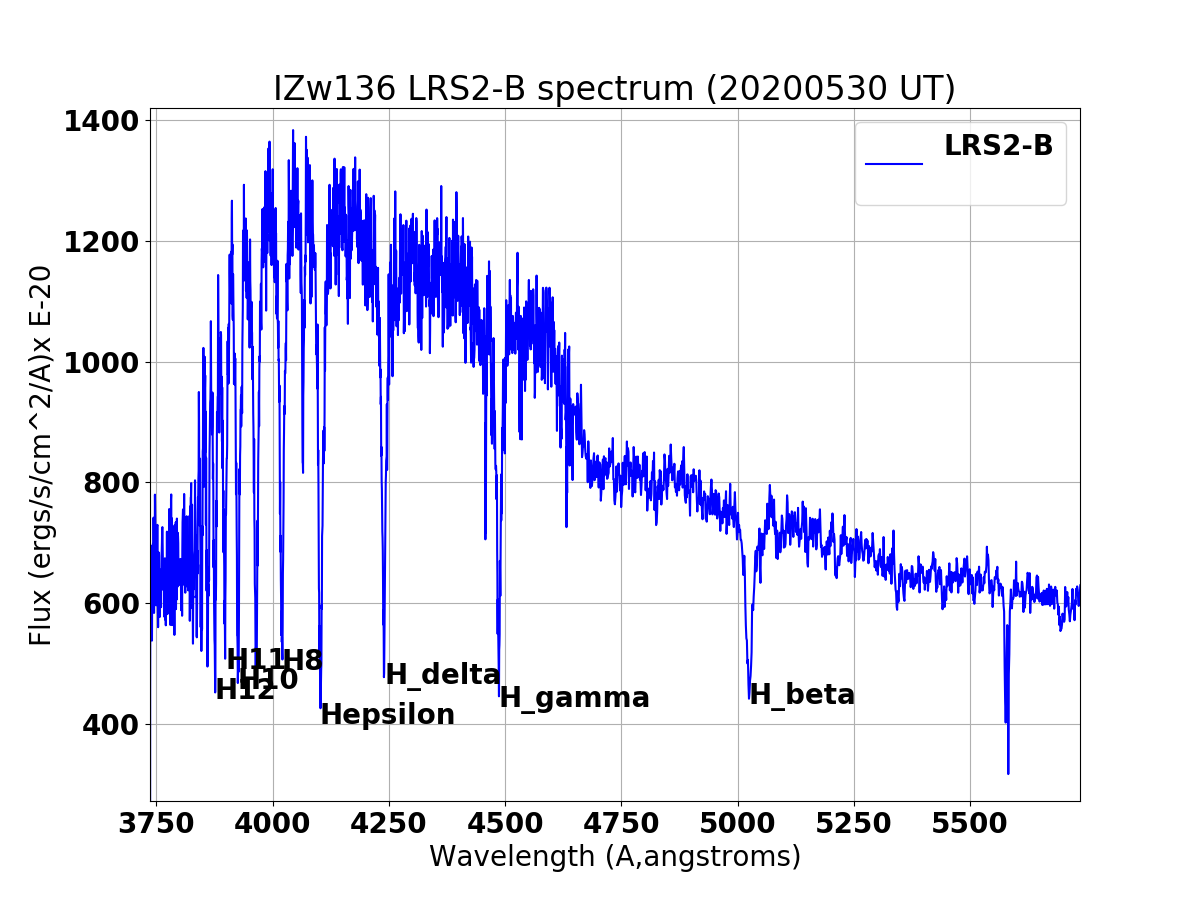A 1-D spectrum from UV and Orange channels of a 20200529 LRS2-B spectrum of 1 ZW 136 (Ra,Dec = 16:13:30.19 +51:03:35.6) is shown. I have identified 8 Balmer absorption lines that are labeled above. The continuum for this specturm appears to be much bluer than for an ordinary E+A galaxy, but the feature identifications seem secure. Rejecting the H_epsilon line, the final table of radial velocity values is shown below Wave_rest Feautre Wave_obs V(km/s) 4101.74 H_delta 4239.69 10082.46 4340.47 H_gamma 4484.69 9960.98 4861.33 H_beta 5023.62 10008.04 3750.15 H12 3875.03 9982.75 3770.63 H11 3897.95 10122.78 3797.90 H10 3924.75 10012.76 3889.05 H8 4018.96 10014.48 Mean Velocity = 10026.3 ± 21.5 km/s mean redshift, z = 0.0334 ± 0.0001

In Aug2020 I spent some time studying up on numpy (see NumPy Studies and in the course of that I developed gregz_002.py (a modified version of a simple GregZ code). I used this to analyza and play with the data cube from Greg that combines the ouv and orange channels into one data cube. I used this two make the two plots below.

 

See notes in /home/sco/jimiL/red_Aug25_2020/Aug25_01/README.red_Aug25_2020
Data cube = eng_galaxy_1_LRS2B_cube.fits
% python gregz_002.py

% cp spectrum.dat spectrum.dat_sco
% vi spectrum.dat_sco                       # just remove header stuff
% cubespec.sh spectrum.dat_sco
Flux min,max = -0.2713111E-15    0.4244979E-15
Enter desired exponent (-14): -19
4727 3 

Resulting file = spectrum.table  (and params,parlab files) 

% mkdir plot1
% cd plot1
% cp ../spectrum.table .
% cp ../spectrum.parlab .
% Generic_Points N
% getrc 
% xyplotter_auto spectrum wave flux 1 N
% xyplotter List.1 Axes.1 N

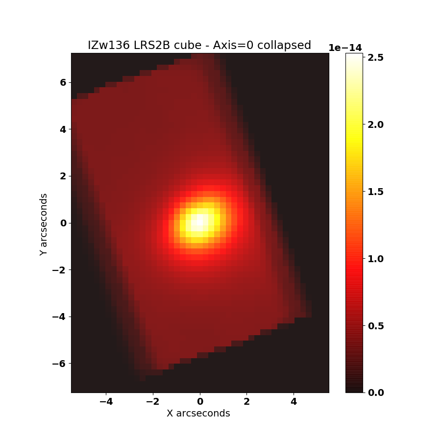GregZ's data cibe (eng_galaxy_1_LRS2B_cube.fits) was collapsed with gregz_002.py to give an integrated light image covering signal from 3640 angstroms to 6949 angstroms.

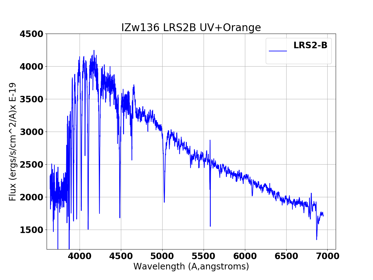IZw136 LRS2-B spectrum extracted with R=1.5 arcsecond circular aperture.