Computing a redshit: Example 1
Updated: Aug05,2020
My input spectrum is assumed to be in the form of a table (i.e. the
files spectrum.table and spectrum.parlab). Just as an illustaration, I plot the
spectrum with my xyplotter_auto routine.
I do this work in:   /home/sco/jimiL/reduce_jul25_2020/Aug05_1

% cat spectrum.parlab
wave    Wavelength (A,angstroms)
flux    Flux (ergs/s/cm^2/A)x E-20
fs      Flux (ergs/s/cm^2/A)x E

% head -7 spectrum.table
# col01: wavelenght in units of angstroms
# col02: flux in units of ergs/s/cm^2/A x E-20
# col03: flux in standard scientific notation, ergs/s/cm^2/A
# data
  3640.00       815.631592       0.81563152E-17
  3640.49       497.090759       0.49709076E-17
  3640.97       716.425720       0.71642576E-17

% Generic_Points N

% cat xyplotter_auto.pars
PointType     L
PointColor    b
LegendName    spectrum
SymbolType    -
Psize         5

% xyplotter_auto spectrum wave flux 1 N
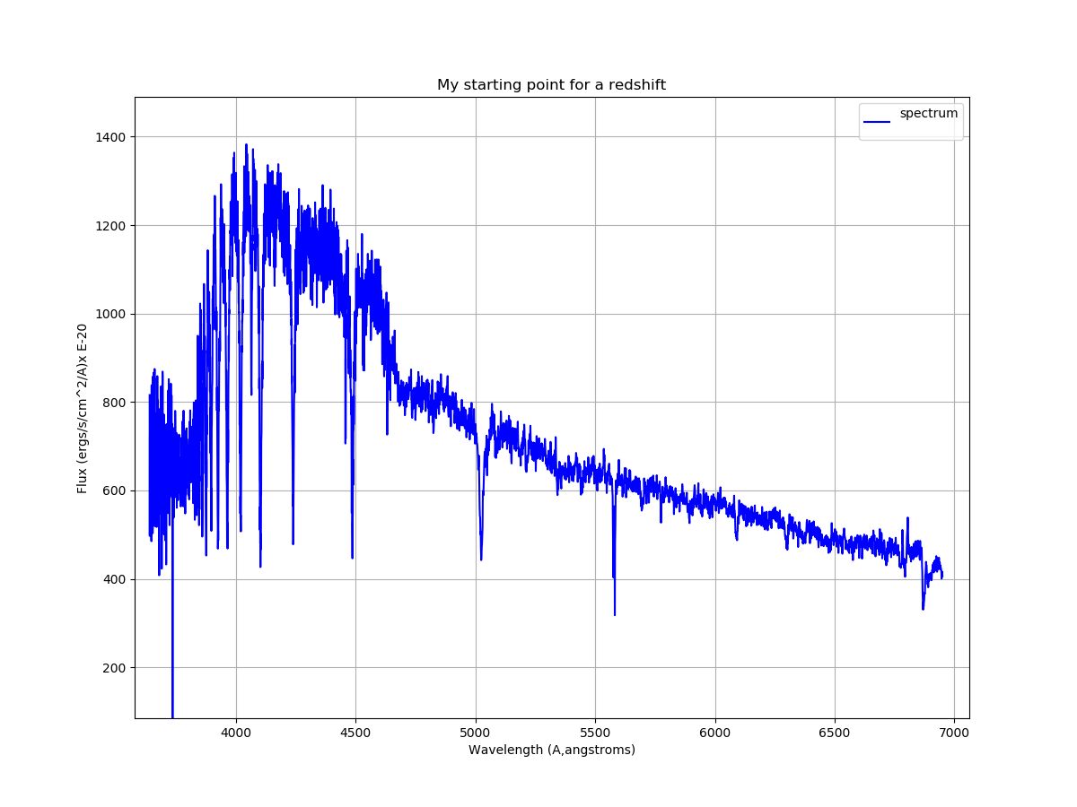 |
Above we see a 1-D spectrum from the UV and Orange channels of LRS2-B taken on
20200529 UT of 1 Zw 136 (Ra,Dec = 16:13:30.19 +51:03:35.6). I am going to guess
that the absorption line little redder than 5000 angstroms is H_beta. I could
"eyeball" from this plot an observed wavelength (Wo) for this line of about
5050 angstroms. Using the implotlib show() option to display the plot I
can get a better estimate of 5023.9 angstroms. With a rest wavelength (Wr)
of 4861.330 angstroms for H_beta we could then estimate a crude radial velocity:
% cat dat.1
5023.9  4861.330  H_beta_L

% redshift.sh dat.1
% cat redshift.out
Initial velocity values:
   Wave_obs     Wave_rest      Feautre            Vobs(km/s)
    5023.900      4861.330     H_beta_L            10025.5
  Mean Velocity =    10025.473     -+       0.000

The formula we used was just:
  v/c = (Wo - Wr) / Wr  , where c is the speed oc light

   v/c  = (5023-4861)/4861 =  0.0333

   v = 0.033 * 299792 km/sec  =  9983.1 km/sec      (or about 10,000 km/sec)
A lot of folks, especially people dealing with very distant HST-observed galaxies,
will use the value of v/c directly. They will refer to this as the redshift, z. Hence, in
our simple calculation here using one identified line we would assign a redshift for 1 Zw 136
of z = 0.033. But what about all those other lines? Can we identify them
and use them to compute a more reilable redshift?
|
Note that I could also have used the routine spec_selector
to view the spectrum and mark the suspected H beta line with an interactive cursor. The resultant
observed wavelength will then be written to a local file named "XY.Mark". Below I show an example
of this.
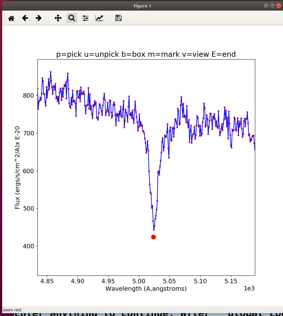 |
Here I plot the same spectrum as above, but I have used "spec_selector" to plot
the spectrum with small red dots connected by blue lines. I zoom in on my suspected
H beta line and mark its position with the "m" key:
% spec_selector spectrum wave flux N
% cat XY.Mark
    5024.411   440.852 m
The big red dot indicates where I marked the observed wavelngth position of the line.
The value we get for our observed wavelength is 5024.4 angstroms, and this agrees
with our previous "spitballing" estimte above.
|
The trick now is to assenble a script or routine that will allow us to run
spec_selector repeated times, identifying multiple spectral features. As
we identify more features we can compute mean radial velocity values to
improve our mean value or to identify unrecognized lines in the spectrum.
I can make a list of spectral lines that might be present in my spectrum.
% speclines.sh ALL 3700.0 7500.0 N
% cat speclines.out
  3727.000  OII_3727
  3934.000  CaII_K
  3968.000  CaII_H
  4101.740  H_delta
  4160.000  CN1_L
  4227.000  Ca4227_L
  4305.000  G_band_L
  4340.470  H_gamma
  4383.000  Fe4383_L
  4455.000  Ca3355_L
  4471.500  HeI_4471
  4531.000  Fe4531_L
  4668.000  Fe4668_L
  4685.680  HeII_4685
  4861.330  H_beta_L
  4958.910  OIII_4958
  4921.900  HeI_4922
  5006.840  OIII_5007
  5015.000  Fe5015_L
  5176.000  Mg_b_L
  5198.500  NI_5198
  5270.000  Fe5270_L
  5335.000  Fe5335_L
  5406.000  Fe5406_L
  5709.000  Fe5709_L
  5754.640  NII_5754
  5782.000  Fe5782_L
  5875.640  HeI_5876
  5893.000  Na_D_L
  6300.300  OI_6300
  6312.100  SIII_6312
  6363.780  OI_6363
  6548.030  NII_6548
  6562.820  H_alpha
  6583.410  NII_6583
  6678.150  HeI_6678
  6716.470  SII_6716
  6730.850  SII_6730
  7065.280  HeI_7065
  7135.780  ArIII_7136
  5577.339  OI_5577sky
  3750.150  H12
  3770.630  H11
  3797.900  H10
  3835.390  H9
  3889.050  H8
  3970.070  Hepsilon
  6867.200  B_fraun_O2
  6276.600  a_O2_6277
Holy moly, that is a lot of lines!
To get a redshift we can use this procedure.
To just get a simple estimate of Vrad:
% cat dat.1
5023.9  4861.330  H_beta_L
usage: redshift.sh dat.1 [-v] [-h]
arg1 - input file listing Wave_obs, Wave_rest, Feature_Name
Additional options:
     -v = print verbose comments and run in debug mode
     -h = just show usage message
% redshift.sh dat.1
   10025.473        0.000    (MeanVelocity,m.e.)

To mark a lot of lines and use them:
% spec_selector spectrum wave flux N
Usage: spec_selector margdist_sub pixel mean N
arg1 - basename of the table file ("Phot_Data" for Phot_Data.table)
arg2 - parameter name for X axis
arg3 - parameter name for Y axis
arg4 - run in debug mode? (Y/N)
**** Make the file   XY.Mark

% redshifter.sh speclines.out 10025.5 -m XY.Mark
usage: redshifter.sh lines.1 29800.0 [-v] [-h] [-m ]
arg1 - input file listing:  Wave_rest, Feature_Name
arg2 - radial velocity in km/s
Additional options:
     -v = print verbose comments and run in debug mode
     -h = just show usage message
     -m = name of a marker file (like XY.Mark from speclines_id.sh) if available
Example:   redshifter.sh speclines.out 10040.800 -m XY.Mark
*** This makes a table named   redshifter.table
To get a final table of data for just the lines with identifications and then
compute final statistics we can follow this procedure:
To get a table of just those lines with identified lines:
% cat rules.1
vrev  fpr  -10 30000.0
% table_mask_builder redshifter rules.1 B0 N
  10     final_number

To get the stats:
% table_stats.sh B0 vrev none N

% table_stats.sh B0 vrev none N
  10013.32  10012.75     68.60      22.86    9887.05   10122.78     9    (mean,median,sigma,m.e.,min,max,N)

I could also use stats_outliers.sh to reject points
Back to calling page