The ability to interact with a simple set of (X,Y) data via an ineractive cursor is very useful.

Mildly helpful matplotlib links.

1. Boston U notes: good quick refs at the end.
2. Ineractive mode 1.
3. A python gythat can write!!!
4. matplotlib doc that is actually useful!.

1. Test data files and a quick demonstration.
2. Version troubles: Dec2018.
3. Interactive mode: An important change!
4. Higher level tools (that work on mcs!)
5. Example: Compute a mean ZP.

An easy demonstration of a cursor code is a good way to start this document.

 

To generate test data:
% make_fit_data poly3 c.3 50 1.0 10.0 0.0 5.0
% colget.py Table1.dat 1 X N
% colget.py Table1.dat 4 Y N
% paste X Y > xy.in
% c3.py 
 

Here are some early notes that briefly describe this test process in mre detail.

 

Early work:   /home/sco/sco/codes/python/cursor/apr6/c3.py   (see README.cursor) 

A) Make the input file (always named xy.in") 

To generate test data:
% make_fit_data poly3 c.3 50 1.0 10.0 0.0 5.0
 Note: the coefficients file (c.3) does not have exist, code will query for values 

Here is a good set of coefficinets: 
% cat c.3
 5.0
 1.0
 2.4

This make a big file:  Table1.dat

To cut out the parts you need for the input file "xy.in": 
% colget.py Table1.dat 1 X N
% colget.py Table1.dat 4 Y N
% paste X Y > xy.in

BTW, to see what type of curve are available:
% gen_curve.sh L 
The first argument to gen_curve is the function 
paramter. Recognized function values are:       
  line    ==  y=a+bx line                        
  polyk   ==  polynomial [k = number of terms]   
  i.e. valid names for a polynomial are:        
  poly1, poly2, ... poly10               
  Example,poly4:   y = a _ b*x + c*x^2 + d*X^4  
  natexp  ==  natural expoenent [y=a*exp(bx)]   
  r4sph   ==  r**0.25 spheroid                  
  gauss3p ==  gaussian (sigma,scale,center)     
 
B) Run the code 
% ct.py 

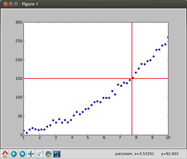The output of my test code ct.py. the code plots a simple set of X,Y data and enables the user to locate X,Y positions in the plot using an interactive cursor. Unfortuantely, as of Jan10,2018, the same code run on mcs does not come out looking like this. The cursor works, but the axis labeleing and the point placement is flawed. The version of python I run on scohome (the version that works) is % python --version Python 2.7.4

In Dec2018 I encountered trouble with running these cursor codes on mcs. This work is described in a set of Dec2018 Version Trouble Notes.

Invoking interactive mode is an important aspect that accomplishes several goals I have been seeking for some time. Using this I can both enter and act upun key strokes in one code. There are still some gotchas. It took me some time to realize that certain keys invoke action. Spme examples are the "s" key causes the Save box to come up, and the "g" key turns the grid mode on. I had to hunt around for keyys that would work well for my pruposes. I assembled a bunch of notes on this stuff. It is worth noting that I show an example of how I make test input file for this code using a gaussioan noise generator named gen_noise. The code to creta the input file named xyf.in is shown HERE.

 

Here is the code:   $codes/python/cursor/icurs4.py 

#!/usr/bin/env python
''' Plot data points read from file xyf.in  and allow user 
    to identify X,Y values using the mouse. The xyf.in 
    file has 3 header lines (title,xlab,ylab) then lines 
    of X, Y, flag where a flag is 0 (plot at red open) or 
    1  (plot as solit blue).  '''

import numpy as np
import matplotlib.pyplot as plt
from matplotlib.widgets import Cursor

# Define the function that will store X,Y values in the 
# the list coords[] when mouse clicks are detected.  
def onclick(event):
    global ix, iy, ib
    ix, iy, ib = event.xdata, event.ydata, event.key

#    print 'x = %d, y = %d b=%s ' % (ix, iy, ib)
#    print 'I have x,y,button' 

# detected END request 
    if ib == "E":
      print "E (END) key was hit"
      quit() 

# detect PICK  
    if ib == "p":
      print "p key was hit"
      plt.scatter(ix, iy, marker="o", color="b", facecolors="b", edgecolors="none", s=70 ) 
      ffc = open('s.key', 'a')
      ffc.write("   %9.3f %9.3f %s \n"  % (ix,iy,ib) ) 
      ffc.close()

# detect BOX
    if ib == "b":
      print "b key was hit"
      plt.scatter(ix, iy, marker="o", color="m", facecolors="m", edgecolors="none", s=70 ) 
      ffc = open('b.key', 'a')
#      ffc.write("   %9.3f %9.3f %s \n"  % (ix,iy,ib) ) 
      ff = plt.axis()
      xb1 = float( ff[0] ) 
      xb2 = float( ff[1] ) 
      yb1 = float( ff[2] ) 
      yb2 = float( ff[3] ) 
      ffc.write("   %9.3f %9.3f %9.3f %9.3f \n"  % (xb1,xb2,yb1,yb2)  )
      ffc.close()
      print "Current X1,X2,Y1,Y2 limits: %s %s %s %s \n" %  ( plt.axis() ) 
      x=[]
      y=[]
      x.append( xb1 ) 
      y.append( yb1 ) 
      x.append( xb2 ) 
      y.append( yb1 ) 
      x.append( xb2 ) 
      y.append( yb2 ) 
      x.append( xb1 ) 
      y.append( yb2 ) 
      x.append( xb1 ) 
      y.append( yb1 ) 
      plt.plot(x, y, "-b")   

# detect UNPICK  
    if ib == "u":
      print "u key was hit"
      plt.scatter(ix, iy, marker="o", color="g", facecolors="g", edgecolors="none", s=50 ) 
      ffc = open('u.key', 'a')
      ffc.write("   %9.3f %9.3f %s \n"  % (ix,iy,ib) ) 
      ffc.close()

# detect MARK 
    if ib == "m":
      print "m key was hit"
      plt.scatter(ix, iy, marker="o", color="r", facecolors="r", edgecolors="none", s=120 ) 
      ffc = open('r.key', 'a')
      ffc.write("   %9.3f %9.3f %s \n"  % (ix,iy,ib) ) 
      ffc.close()
#      quit() 

    global coords
    print "after   global coords   statement\n",
    coords.append((ix, iy, ib))
    print "after append \n",
    if len(coords) == 100:
        fig.canvas.mpl_disconnect(cid)
    return coords

def onclick2(event):
    print('%s click: button=%d, x=%d, y=%d, xdata=%f, ydata=%f' %
          ('double' if event.dblclick else 'single', event.button,
           event.x, event.y, event.xdata, event.ydata))

#=========================================================
# Here is a sample xyf.in file that you can test with 
# Test data for icurs3.py
# X axis title 
# Y label string 
# 1.0  1.0  0
# 2.0 2.0   0
# 3.0 6.0   0
# 4.0 4.0  1
# 8.0 8.0   0
#=========================================================

#=========================================================
# read the the X,Y plot data from file xy.in for reading 
infile = open('xyf.in','r') 
# Read axis label info
header1 = infile.readline()
header2 = infile.readline()
header3 = infile.readline()
label_main  = header1.rstrip()
label_xaxis = header2.rstrip()
label_yaxis = header3.rstrip()

# Gather the X,Y values and the current flag values
# flag=0 point is not selected 
# flag=1 point is selected 
x = []
y = [] 
f = []
xs = []
ys = []
for lines in infile:
 linefull = lines.split()
 x.append( float(linefull[0]) )  
 y.append( float(linefull[1]) )  
 f.append( linefull[2] )  
 if linefull[2] == "1":
  xs.append( float(linefull[0]) )  
  ys.append( float(linefull[1]) )  
infile.close()

# Give some info 
nsel = len(xs) 
print "\nNumber of flagged (=1) points = %d \n" % (nsel),

# Debug lines 
nxp = len(x) 
print "Number of X,Y points read from xyf.in = %d\n" % (nxp) 
#print "Here are the X,Y points read:\n" 
#i=-1
#for lines in x:
# i=i+1
# print " %12.4f   %12.4f   \n" % (x[i],y[i]), 
#
#any = raw_input("\n\nEnter anything to continue: ") 

#=========================================================

#=========================================================
# experimental
paramso = {'savefig.format'       : 'png',
          'figure.figsize'       : [9.0, 9.0],
          'font.size'            : 15,
          'axes.formatter.limits': [-3, 3]}
plt.rcParams.update(paramso)
#=========================================================

# Turn interactive mode on
print "ready to turn interactive mode ON. \n",
plt.ion()
print "interactive mode is ON. \n",

# Plot the data 
fig = plt.figure()
ax = fig.add_subplot(111)

#plt.scatter(x, y, marker="o", color="r", facecolors="b", edgecolors="r", s=70 ) 
plt.scatter(x, y, marker="o", color="r", facecolors="none", edgecolors="r", s=70 ) 
plt.scatter(xs, ys, marker="o", color="r", facecolors="b", edgecolors="none", s=70 ) 
print "plt.scatter was run. \n",

# Make a red, two-line cursor
print "ready to Cursor run. \n",
cursor = Cursor(ax, useblit=True, color='red', linewidth=2)

# Set up the coords list for storing X,Y at click positions 
coords = []

cid = fig.canvas.mpl_connect('button_press_event', onclick)
cid2 = fig.canvas.mpl_connect('key_press_event', onclick)
#Zcid = fig.canvas.mpl_connect('button_press_event', onclick2)

# label the axes
print "ready to label axes. \n",
label_m = "Keys to use:  p=pick  u=unpick   m=mark    E=end "
plt.title(label_m)
plt.xlabel(label_xaxis)
plt.ylabel(label_yaxis)

#plt.draw()
#plt.show()

any = raw_input("Enter anything to continue: ") 
# Coords is a list of lists 	
print "I will print coords here: "
type(coords)
c=len(coords) 
print "Number of x,y sets (mouse clicks) collected in coords = %d" % (nc)
# Open a file for saving header lines
fcurs = open('cursor.lines', 'w')
print "\nHere are the stored mouse click events:"
for i in range(0,nc):
  s = coords[i]
  fcurs.write("   %9.3f %9.3f %s \n"  % (s[0],s[1],s[2]) )
fcurs.close()

In practice, we want some general routines that simplify the use of our interactive cursor. Also, as discussed in the rpevious section, we want these tools to work correctly with different python versions.

One of the firt practical uses of my python routine icurs1.py was used to compute mean photometric zeropoints. You can read about this in discussion of reducing a night of acm data). Briefly, I wanted to isolate a group of ZP points in an X,Y plot and compute a mean value with a few other useful statistics. I developed table_xy_boxclean for this. I use my cursor to set a bottom-left corner (BLC) and a top-right corner (TRC) in the XY plot. I can then isolate the box member points and compute my statistics.

 
% ls 
 margdist_sub.parlab margdist_sub.table
% table_xy_boxclean margdist_sub pixel mean N
% ls
margdist_sub.parlab     margdist_sub.table         table_xy_boxclean.X  table_xy_boxclean.Xstats  
table_xy_boxclean.Y     table_xy_boxclean.Ystats

A new version that uses (as of Dec30,2018) icurs4.py. This versions used the interactive mode in matplotlib, and hence is much more effiecient from the standpoint of the user.

 
% ls 
 margdist_sub.parlab margdist_sub.table
% table_point_selector margdist_sub pixel mean N