1. Measuring sky surface brightness.
2. The basic recipe for a single acm night.
3. The basic recipe for multiple acmnights. (OBSOLETE)
4. Survey multiple nights.
5. Clouds: Is a night worth reducing?
6. Obtaining bias and dark frames at the telescope.
7. Removing the acm bias and fixed bias pattern (FBP).
8. Buildng a master dark rate frame.
9. Initial CCD processing.
10. Visually checking a lot of acm images.
11. Analysis of acm image reults.
12. Appendices: A variety of docs related to acm processing

The motivation for this document centered around measuring night sky surface brightness values with the acm. The bias, and to a lesser extent the dark levels, must be subtracted before we can measure a mean flux level due to the sky signal. Some early numbers from an analysis of sky frames indicate that if we assume a bias uncertainty of &pm 6 adu (if no bias fraem are available for a given night) then our sky flux uncertainties will be 11% and 3% in g,r respecticvely. The derivation of these estimates is described in a quick first look at g,r sky levels..

A primary goal of this work was to measure night sky surface brightnees values with the acm using differential photometry from stars in ean acm field. Here are some quick notes.

 
 
# Use https://www.google.com/  and search on "dark sky g band sky brightness"

http://www.ctio.noao.edu/noao/node/1218
 *** Lots of good references and these mean values: 

U 	22.12 mag arcsec-2
B 	22.82 mag arcsec-2
V 	21.79 mag arcsec-2
R 	21.19 mag arcsec-2
I 	19.85 mag arcsec-2
u 	23.3 mag arcsec-2
g 	22.3 mag arcsec-2
r 	21.4 mag arcsec-2
i 	20.5 mag arcsec-2
 

The very basic reduction recipe for processing a single acm night is given here. The details are discussed in Treating one acm image. I usually run the initial steps on mcs to create a smaller subset of images for reduction: the bias images and the "viable" open sky images. By "viable" I mean images with enough stars present to allow a WCS and ZP derivation. Typically the first step in any acm treatment is to survey the properties of the acm images using acm_table_markII.

I specifiy the night with the local files: 
BaseDir     (usually /hetdata/data on mcs) 
Date        (YYYYMMDD) 
% acm_table_markII N                          # fast method using only headers 
% point_selector ACMDAT uthrs im N            # Visually select good sky images  

NOTE: Since the data are directly accessed only (?) from mcs, I do these 
      steps in:   /home/mcs/sco/ACM_reds_2/Raw_Subsets
      There I have the file README.quick which gives a terse guide. 

 
Older way of doing things on mcs: 
[sco@mcs Raw_Subsets]$ cat README.quick
acm reductions (quick) 
=======================
% acm_table 10.0 N                               # ACM table 
% acm_table_qc ACM Y N                           # makes list.* files, including list.BIAS 
% point_selector ACM timeH ImNum  N
% mkdir acm 
% cd acm
% cat ../list.BIAS ../Viewed.Images >list.pull
% impuller list.pull
% \rm -r ../local_red/BASIC
 

 

I specifiy the night with the local files: 
BaseDir     (usually   /media/sco/DataDisk1/sco/AD/HET_work/acm_raw_subsets) 
Date        (YYYYMMDD) 
% acm_table 10.0 N                            # ACM table 
% acm_table_qc ACM Y N                        # makes list.* files, including list.BIAS 
% acm_bias_for_date 20190207 N                # prepare bias correction files 
% acmred_list list.OPEN N  

1. Preps FITS header, subtracts bias and dark signal.
2. Derives WCS and installs in FITS header
3. Derives ZP (photometric zeropoint) and installs in FITS header
4. Derives sky surface brightness and installs in FITS header

I discovered that when I attempted to reduce older (early 2018) acm images, the astrometry pipeline failed becasue the raw acm images have faulty headers (i.e. ds9 or xy2sky will not report RA,DEC values). A quick fix was found for these cases:

cd /media/sco/DataDisk1/sco/AD/HET_work/acm_raw_subsets/20180109/acm
sethead -k RADESYS='FK5' 201*.fits

Using this procedure I reduced acm images for the night of 20190207. This was a day after new moon, and the Boston allsky image site reveals the night was extremely clear all night long. Of the 12 reasonable sky images, 7 had enough stars for good WCS determination (and hence photometric zeropint calibration by cross-matching to PANSTARRS) For these 7 images I derive a mean g band sky surface brightness of:

 
 mean(mu_sky in g) = 22.336 -+0.049 mss      (median = 22.384 mss)
 where mss = magnitudes per sq.arcsec

For refence, here are some mean values from Kitt Peak for clear, moonless
nights:
g       22.3 mag arcsec-2     *******
r       21.4 mag arcsec-2
i       20.5 mag arcsec-2

The mean ZP for a 1 -sec exposure, with no correction for pupil filling, is: 
   = -2.34663 -+ 0.03217  (7 images) 

The very basic reduction recipe for processing sets of acm nights is given here. By "processing" we mean the acm image headers are repaired and the bias and dark signals are removed. However, no subsequent reduction (WCS, ZP, SKYSB) is performed.

Survey the acm images for multiple nights:   
% cat BaseDir
/home/sco/AD/HET_work/acm_nights
NOTE:  The do_acm_night script requires the BaseDir file be placed in ./S/BaseDir 
% head -3 list.Date
20170906  
20171129  
20171231  
% acm_nights list.Date /home/sco/AD/HET_work/acm_nights N
# If a local BaseDir file is present, then use: 
% acm_nights list.Date none N  

To process images from multiple nights   
% acm_BigRed list.Dates N N  
arg1 - Name of file with list of UT dates to be processed 
arg2 - Allow interactive query of user (Y/N) 
arg3 - run in verbose/debug mode 

*********    WORK IN PROGERSS  ************
=======================================================================================
*** After I have processed all of the nights, I can investigate dark frames 
In each date directory:
  image_fullpath_list list.DARK FIXUP list.dset N        # wrote dlists.bash to do this
Then I cat these into:   list.BIGDARKS
    # cd ./Dark_study_1/ ; cat ../20*/list.dset > list.BIGDARKS
Then I build the table of dark image data
  acm_dark_table list.BIGDARKS N
I can then use point_selector on the DARKS table file
For examples:   point_selector DARKS exp drate1 N 
                Generic_Points ;  xyplotter_auto DARKS q q 20 N 
=======================================================================================

I have begun periodically running acm_nights on mcs to survey large sets of nights. I am collecting the results of these acm_runs here.

In trying to outline how we reduce a single night of acm images I uncovered a host of problems. To treat many of these required me to inspect and compare image properties from many nights. To more easily summarize many nights of data I developed the routine acm_nights. Basically I want use a file that lists the dates I am interested in, and the location on disk where my date subdirectories are located (for example, on mcs we usually used /hetdata/data). In the file "list.Date_1" for the example below I listed the date strings for nights of interest. The second argumnet can be the base directory of the data sets, but if a local BaseDir file is present, this address is taken from there. Here is a brief example:

  
% acm_nights list.Date_1 none N 
% cat acm.nights_SUMMARY
Basepath used  = /media/sco/DataDisk1/sco/AD/HET_work/acm_nights
Number of nights to be surveyed  = 10
  Date         Nimages     Nbias    Ndark     Nopen   Nnone  Moon_illum
  20190128       346         0         0       336       10    48.900
  20190204       351         5         0       336       10     0.700
  20190205       771        32         5       463      271     0.000         # A good night? 
  20190206        97        28        63         6        0     1.200
  20190207       295        25         0       270        0     4.100
  20190216       373         9         0       354       10    81.500
  20190217       585        11        12       552       10    89.700
  20190218       300         7         0       283       10    95.800
  20190219       113        56        57         0        0    99.300
  20190302       509         0         0       497       12    18.300
Processing time for these nights = 54.000000 (seconds)

 
 
 if [ $nims != "0" ]
 then
  acm_image_table list.IMAGES ACMDAT N
  acm_table_qc ACMDAT N N > out.qc
  read nbias ndark nopen nnone comment < out.qc
 fi
 printf "  %8s    %6d    %6d    %6d    %6d   %6d\n" $date $nims $nbias $ndark $nopen $nnone | tee -a $fo

 
 
[sco@mcs ~/ACM_reds_2]$ pwd 
/home/mcs/sco/ACM_reds_2

[sco@mcs ~/ACM_reds_2]$ ls -1 /hetdata/data > dates.4      
# I edit dates.4 to contain only 2018,2019 dates  

[sco@mcs ~/ACM_reds_2]$ ls 
BaseDir  dates.4

[sco@mcs ~/ACM_reds_2]$ fast_acm_nights dates.4 N 
   

A lot of effort can be expended reducing a night of acm data only to learn later that any photometric analysis has been compromised by clouds.

 
 
http://sirius.bu.edu/dataview/     # Boston site 
https://lco.global/camera/elp/allsky/archive   # LCOGT camera, images kept 24 hours 

For Boston images:   
 * I use the 6950 images (shows clouds well)
 * Date seems to be UT dates 

 

From the table above made with acm_nights, we see that the night of 20190205 had bias images and large number of open sky images on a nearly moonless night. The Boston image data base, however, shows that there were intermittent clouds throughout the night. Below is a figure that illustrates some of the Boston images. Here it is.

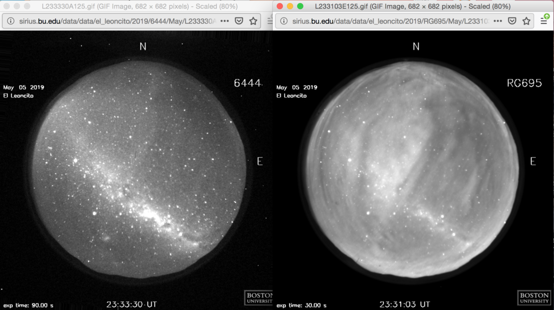Samples of Boston all-sky camear images. I have been using the 6950 images for assessing clouds, but there could be reasons to use other filters if they are available. Note from Joei Wroten about this image: The sky monitoring filters we use are 6444 or 6050. This is outside my area of "expertise", so I'm going to be general here, but 6950 can show some mesospheric activity that could be deceiving on a clear night. I'm going to attach an image from one of our other sites that illustrates this nicely (southern hemisphere sky). The image on the left is 6444 and is clear with lots of stars visible. The image on the right is 6950 and taken just a couple minutes earlier. That's the mesophere, not clouds, in 6950. But it's true that certain clouds can look very obvious in 6950.

In conclusion, even though the night of 20190202 had bias frames, lots of sky images, and was very close to new moon, this would not be a good night for assessing sky surface brightness. Both the 6050 and 6950 images showed many clouds in most of the images throughout the night.

As well see in the following sections of this document, the bias and dark levels of the acm appear to be variable. At this time (Jan2018) it remains unclear if this variability is a function of temperature or some other property. To help eliminate some possibilities I have prepare several scripts that should be used observers to obtain the bias and dark frames for acm. This scripts handle things like insuring that light-emitting sources, like the PV camera, are powwered off and that the FCU head is deployed abd the acm mirror is retracted. All of thses measures are designed to insure that unwanted sources of scattered light will not reach the acm when bias and dark images are being taken. Here are the commands the RA should use:

 
# Take 43 acm bias frames    
% acm_bias_run 43 
arg1 - number of bias images to take  

# Take 21 5-second acm dark frames    
% acm_dark_run 21 5  
arg1 - number of images to take  
arg2 - integration time (5, 10, 20) 

The bias level must be subtracted from any acm image if we are to derive valid sky surface brightness estimates. The acm has a very significant fixed bias pattern (FBP) and this must be removed in order to greatly reduce the field noise in a raw image. These topics are discussed in acm bias properties. In practice, as of May2019, the easiest way to assemble to data needed to perform a bias correction of the acm images can be performed with:

 

% acm_bias_for_date 20190217 N  
Usage: acm_bias_for_date 20190217 N  
arg1 - date of night to be run (YYYYMMMDD) 
arg2 - run in debug/verbose mode 

The mean dark rate for the acm, when using exposure times of 20 seconds or less seems to be around 0.5 adu/sec. Details and figures are given in this discussion of dark frame properties of the acm.

Now that we hav covered how to summarize the acm images available for one or more dates, and we have covered how to build basic CCD processiong images like biax frames, fixe bias patter (FBP) tabls, and dark frames, we can processed to perform the initial processing on the acm images from selected nights. A simple recispe for reducing three nights is given below.

 

# Specify where the raw data are stored and which night are to be processed 
% cat BaseDir
/home/sco/AD/HET_work/acm_nights

% cat head -5 list.Date
20170903
20180402
20190219

% acm_BigRed list.Dates N N  
arg1 - Name of file with list of UT dates to be processed 
arg2 - Allow interactive query of user (Y/N) 
arg3 - run in verbose/debug mode 

Sometimes one simply wants to process a single image. This can be done with the pasa script. The bias data for a given night can be assembled with the acm_bias_for_date script. I show an example below of a typical acm processing with pasa.

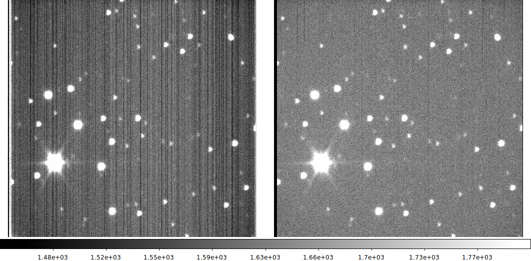An example of a raw acm image (left) after ccd processing (right). This is a ramdom acm image from the night of 20190505. This image has been processed with teh pasa code. A fixed bias pattern (FBP) and a mean bias level has been subtracted. A sclaed dark rate image was also subtracted.

It is very useful to be able to quickly view a lot of acm images. I have two basic approached: one that uses ds9 to view large numbers of tiled ds9 images, and one that uses a plot package with an interactive cursor that allows one to select an point in some parameter space and view the corresponding image in a ds9 window. These approaches are described in detail in this discussion of acm image display packages.

The initial analyses use manual table file methods to assemble FITS header information (from images processed through the SKYSB phase) and produce various plots. I am assembling a collection of acm photometry analyses.

A host of early notes and links to useful documents have been compiled in an Appendix Section. The first entry of this Appendix section is a 2018 of this document.