Treating a single acm image.
Last updated: May14,2019
Just show me the recipe.
% cat ./BaseDir
/media/sco/DataDisk1/sco/AD/HET_sco_tests        # Image base directory on sco2019
/media/sco/DataDisk1/sco/AD/HET_work/acm_raw_subsets    # Image directory collected on mcs

% cat Date
20190207

# To get useful working lists and ACM table
% acm_table 10.0 N
% acm_table_qc ACM Y N
**** A list of good sky images is in:    list.OPEN
WARNING: Run acm_table in a clean directory so that it does not
         get confused by images present in a pre-existing
         ./local_red subdirectory.

# To prepare bias files
% acm_bias_for_date 20190207 N

# To see the images in a 4x4 grid and pick images
% bigds9 list.OPEN 16 16
**** Images I mark show up in:   big.MARK
% cat big.MARK
/media/sco/DataDisk1/sco/AD/HET_work/acm_raw_subsets/20190207/acm/20190207T081631.3_acm_sci.fits

# CCD correct, WCS- and ZP-calibrate, and measure SKYSB for a single image
% acmred /media/sco/DataDisk1/sco/AD/HET_work/acm_raw_subsets/20190207/acm/20190207T081631.3_acm_sci.fits N


# Recall that the individual steps run by acmred are:
% pasa /media/sco/DataDisk1/sco/AD/HET_work/acm_raw_subsets/20190207/acm/20190207T081631.3_acm_sci.fits Y N
% wcsf ./local_red/FIXUP/20190207T081631.3_acm_sci.fits N
% zpmido ./local_red/WCS/20190207T081631.3_acm_sci.fits N
% sb_mido ./local_red/ZP/20190207T081631.3_acm_sci.fits N
Introduction: what is to be done.
Sometimes we want to quickly reduce a single acm image. The term "reduce" can mean different
things. It could mean just applying bias corrections, derive WCS and/or photometric ZP values,
or it it could extend to the estimation of a calibrated sky surface brightness or other measurement.
Test data: HET_sco_tests.
I have collected some representative acm data sets that can be used for quick demonstration
and development purposes. I usually place HET_sco_tests in a directory names AD = All Data)
on most of the machine I use.
/home/sco/AD/HET_sco_tests
20190217 = collection of bias and sky images from one night
20190401 = a single acm image with many stars (no bias data)

Here are the sky images:
/home/sco/AD/HET_sco_tests/20190217/acm/20190217T022612.7_acm_sci.fits
/home/sco/AD/HET_sco_tests/20190217/acm/20190217T032400.6_acm_sci.fits
/home/sco/AD/HET_sco_tests/20190217/acm/20190217T105816.6_acm_sci.fits
/home/sco/AD/HET_sco_tests/20190217/acm/20190217T122456.6_acm_sci.fits
/home/sco/AD/HET_sco_tests/20190401/acm/20190401T115437.0_acm_sci.fits    # Very dense star field

A typical BaseDir file to access these images for a test reduction:
% cat ./BaseDir
/home/sco/AD/HET_sco_tests

On my new machine at home (sco2019):
/media/sco/DataDisk1/sco/AD/HET_sco_tests

On a typical mcs reduction:
/hetdata/data
CCD processing.
The simplest reduction is just basic CCD processing and interactive viewing of the image.
First, I use an easy way to assemble the bias information for this night:
% acm_bias_for_date 20190217 N
  arg1 - date of night to be run (YYYYMMMDD)
  arg2 - run in debug/verbose mode
** This creates a lot of stuff in ./bais, but the local files we need for further
   processing are:   BIAS.DATA , fbp.table

To push an acm image through basic CCD processing steps:
% pasa /media/sco/DataDisk1/sco/AD/HET_sco_tests/20190217/acm/20190217T122456.6_acm_sci.fits Y N
  arg1 - name of acm image (can be full path)
  arg2 - run in interactive gui mode mode
  arg3 - run in debug/verbose mode
Note that the files named BIAS.DATA and fbp.table could now be used for reducing any other
acm night. For instance, in the case of 20190401 I save only the single sky image of
interest for the test data directory. Using the 20190217 to reduce 20190401 is preferable
to using the $critfils default version from 2018-04-02. The figure below illustrates a
typical image processing result with pasa.
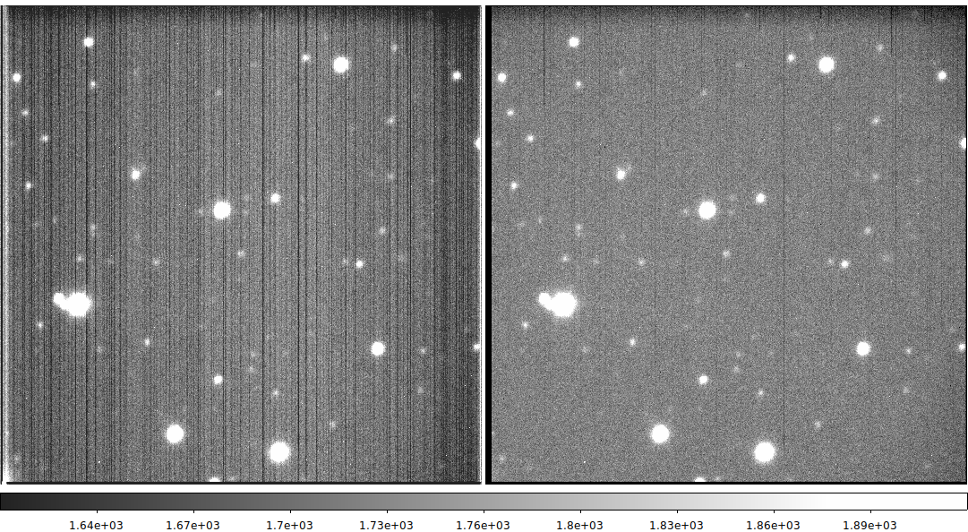 |
Processing of a typical acm image by pasa. The raw image is shown in the left panel.
After cleaning of the FITS header, the significant fixed bias pattern was removed
(using fbp.table). The mean bias signal (read from BIAS.DATA) was subtracted. A mean
dark rate image (from the $critfils directory) was used to subtract the dark signal.
The final image was deposited in the ./local_red/FIXUP directory. Notice that the fixed
bias pattern is well-removed , as is the small dark signal feature in the lower-left
corner of the raw image. The dark vinetting features, most noticable in the upper right,
are not removed. The acm illumination correction is strongly dependent on tracker X,Y
position, and hence, is not easily corrected.
% cat ./BaseDir
/home/sco/AD/HET_sco_tests
% acm_bias_for_date 20190217 N
% pasa /home/sco/AD/HET_sco_tests/20190217/acm/20190217T122456.6_acm_sci.fits Y N
% ls ./local_red/
FIXUP/	HDFIX/	RAW/
% ls ./local_red/FIXUP
20190217T122456.6_acm_sci.fits
The next downstream reduction script will use the image in ./local_red/FIXUP, but
the intermediate image versions in RAW and HDFIX are stored.
|
WCS calibration.
The goal is to assemble a single, user-friendly script for installing WCS. This will
incorporate four wcsf_ codes. You can read a recipe for
using the wcsf codes.. It is worth noting that most of the internal parameters used
by these wcsf_ codes can be set with a local file named "WCSF.DEFAULTS". You can
build such a file with the routine wcsf_defaults.
All four wcsf_ codes can be run on a single image with wcsf:
% wcsf ./local_red/FIXUP/20190217T122456.6_acm_sci.fits N \n"
Briefly, the role of each wcsf_ code run by wcsf is:
- wcsf_rough: Use ds9 to identify a DSS
star in the field and derive a rough (good to an arcsecond) WCS for the image header.
- wcsf_viscat: Use ds9 to confirm that the rough
WCS is valid and establish a suitable USN-B1.0 catalog of astrometric stars for further redcution.
- wcsf_imgcat: Use image thresholding to detect
sources and establish a catalog based on image moments.
- wcsf_final: Cross-macth the image moments catalog with
USNO-B1.0 to establish a larger set of fitting data. Derive a revised WCS solution with errors.
ZP calibration.
You can read about the steps in developing a
zeropoint tool, but the basic procedures we need to perform are listed
below. With a FITS image that has a good WCS calibration in the header,
the problem of deriving a phtometric calibrayion (i.e. for mag =
ZP - 2.5log(Flux) we want to determne the value of ZP) should be as
simple as:
- Compute instrument magnitudes (magI) for sources on the image
- Query a catalog like PANSTARRS (PS1) to get standard magnitudes (magS)
in the area of our image
- Positionally cross-match these two catalogs and compute
ZP = magI - magS for every available source
- Reject bad points and compute a mean value and error for ZP.
Do all of the above and more with zpmido:
A good practice location: /home/sco/tmp/ZP_work2
Note that I use as inoput the path to a WCS-calibrated image.
% zpmido /home/sco/tmp/local_red/WCS/20190217T122456.6_acm_sci.fits N
At the end of this procedure we'll have a local version of the image
that has ZP-related header cards installed in the FITS image. Here is
an example (as of May04,2019):
% imhead ./20190217T122456.6_acm_sci.fits
The relevant line:
ZPSEC   =              -3.1620 / ZP for a 1-sec exposure
ZPERR   =               0.0382 / mean error of ZPSEC
NUMZP   =                    7 / number of calbrating sources
PSYSNAME=                    i / name of photometric system
In words, this gives the zeropoint for transforming a 1-second exposure to
the phtometric system given by PSYSNAME. The number of calibrating sources
(n=7 above) is useful in judging how realistic the estimated zeropoint
error (ZPERR) should be considered.
Be warned that the python code (ps1.py) that retieves the PS1 (panstarrs) data is a
little klunky. It writes the gri photometry with a fixed format, and in some cases
a star may not have one of these values. The code throws warnings to the user in cases
of "nan" (not a number) events. I'll try to fix this eventually. The error that appears, and
can be ignored for now, is:
['objID', 'RAJ2000', 'DEJ2000', 'e_RAJ2000', 'e_DEJ2000', 'gmag', 'e_gmag', 'rmag', 'e_rmag', 'imag', 'e_imag', 'zmag', 'e_zmag', 'ymag', 'e_ymag']
/home/sco/Installs/install_sco2019_20190511/bin/python/ps1.py:87: UserWarning: Warning: converting a masked element to nan.
  ffc.write(" %12.8f %12.8f  %7.3f %7.3f %7.3f \n"  % (ra,dec,gmag,rmag,imag) )
Sky surface brightness estimation.
You can read about the steps in deriving a
mean sky surface brightness. The routine to implement this is shown below:
%  skysb_mido 20190217T122456.6_acm_sci.fits N

The relevant header cards instlled here:
RSTRT   =           -1050.6305 / Radius position of tracker at start (mm)
MILLUM =             -99.0000 / percentage moon illumination
PHIMOON=             -99.0000 / angle of separation to moon (deg)
VSKYSB =              21.9000 / predicted V sky surface brightness
SKYSB   =              19.6607 / sky surface brightness (mags per sq.arcsec)
SKYSBERR=               0.0038 / mean error of SKYSB
NUMBOX  =                    7 / number of sky boxes measured
Back to calling page