In this document we'll cover how to view the contents of an image file. Originally I began this document with the ide of just covering the use of xpa to run ds9. When I began searching for ways to make images with overplotted information, particularly markers having to do with important spatial information (positions of star, N-E legend, plate scale legend, etc...) I began to see that ds9 was limited. Actually, you can do a lot of the operations with ds9, but if you want to do something like make a more standard image format (like png) with ds9, and then pretty it up with other graphics packages, you hit some fundamental problems that (as of June2015) I have been unable to solve. Hence, I added some sections on making image plots with python (specifically matplotlib) and the seemingly pervasive ImageMagic package.

1. Astronomical image files.
2. Using ds9 and xpa.
3. Using ImageMagic.
4. Using python: matplotlib and other things.
5. A mix of things for VIRUS.
6. Nov2015 Commissioning Run.

The basic image file format we'll see most in astronomy is a FITS files. The ds9 display code is designed to handle FITS images, and the xpa code is designed to communicate with the ds9 window. By communicate, I mean your can execute ds9 commands from your script or program that allow you to interact with your image. In this little intro section I show some things we can do with a test image of NGC3379 (named n3379_B.fits). All of this was done in my Test_Data directory: $tdata/T_runs/Image_Render/ex0_n3379.

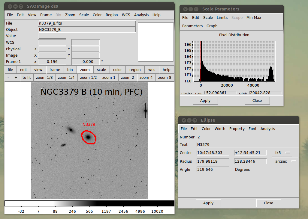Here we use ds9 to view the image of NGC3379. I have run ds9 in a manual mode here and I opened the Scale window so that I could view the histogram of pixel values and establish a better grey-scale image. I also marked an ellipse region and I opened the region window that describes that ellipse. Because the input image has WCS parameters in the header, I can have the ellipse (or any cursor properties) expressed in units like RA, Dec, arcseconds, etc.... as well as he usual simple pixel values. This is a major strength of ds9, it can use a lot of the useful information present in FITS headers. Finally, note that I made the html text for this spiffy figure using: build_htm_img ds9_manual.png ds9_manual.txt > my_html

I have written and collected a lot of tools that can operate with FITS files. Below I show few snippets of code that take our NGC 3379 image above, and create a png (Portable Network Graphic) image file. I use xpa commands from within a script to run ds9. The ds9 graphic above took about a minute to execute. The one below took about a second. Moreover, I can use this approach to compile a very complicated image construction sequence, and use it over and over. Just bewause it is useful, I show below how I used the getfits tool (from wcstools) to cut out a small portion of the NGC3379 image for this plot. My little script (called "doit") wants is hard-coded to use this sub-image (called sub.fits) to create a png file (which I show you below).

 

% getfits -o sub.fits n3379_B.fits 420-1020 740-1340
Row  1339 extracted   
sub.fits

% ccdsize sub.fits
601 601

% doit 800 800
Enter any key AFTER ds9 window opens.
DS9 ds9 gs 7f000101:43417 sco
User z2 = 519.300
c_sub_800_800.png PNG 800x653 800x653+0+0 8-bit DirectClass 440KB 0.000u 0:00.000

Here are the guts of "doit": 
#!/bin/bash
# Check command line arguments
if [ -z "$1" ]
  then
    printf "Usage: doit 500 700\n"
    printf "arg1 - X size\n"
    printf "arg2 - Y size\n"
    exit
fi
ds9_open $1 $2
ds9_views_off
imlook sub.fits 30
xpaset -p ds9 saveimage c_sub_$1_$2.png
identify c_sub_$1_$2.png

Finally, just for completeness I will identify all three of the bright galaxies in the rather lousy PFC image I am using here in this exercise. Note that I use eye-ball settings of region markers to create a regions file for the three galaxies and list their Ra,Dec according to the image WCS. As a sanity check on the getfits code (i.e. to insure that it is still preserving WCS properly) I list the ds9 equatorial coordinates I derive from the sub.fits image.

 
                NED Coordinates (J2000)            Image WCS                  Sub_Image WCS 
              --------------------------   -------------------------   -------------------------
NGC3379 (E)   10h47m49.588s +12d34m53.85s  10:47:49.485 +12:34:54.07   10:47:49.485 +12:34:52.72
NGC3384 (S0)  10h48m16.886s +12d37m45.38s  10:48:16.628 +12:37:44.03   10:48:16.720 +12:37:45.39
NGC3389 (Sp)  10h48m27.910s +12d31m59.50s  10:48:28.029 +12:31:51.33   10:48:28.305 +12:31:54.05

For the full image:  n3379_B.fits
                X_image  Y_image 
NGC3379 (E)      974.0   1055.5
NGC3384 (S0)     680.0   1180.5
NGC3389 (Sp)     557.0    925.5

Finally, for the full image, I can draw a large circle 
that goes through the centers of {NGC3379,84,89} with:
 
  CENTER :   Ra,Dec=10:48:08.297,+12:33:20.00     X,Y=(771.0,986.5) 
  RADIUS =   292.7 arcsec   ,    216.1 pixels 

 

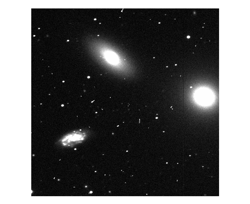
Here is the image of NGC3379 using the doit script described above. As we'll see later in this document, I can use xpa to make all sorts of adjustemnts, and then create a more general image file (like png, tiff, jeg,...). However, one problem that I have encountered is evident above. The user specifies the size of the entire ds9 gui (800x800 above), but the image is displayed in the viewing windo area, and I have been unable to learn how one can query or set this size. The problem arises because when we dump and image file (using saveimage in ds9), the ENTIRE viewing window is dumped, including all of the surrounding white-space! As we'll see later in this document, this complicates the process of using other method (like a python script) to over-write things on our image file. Such is life.

Finally, I can take a file like the png image we generated above and spiff it up using the python matplotlib package:

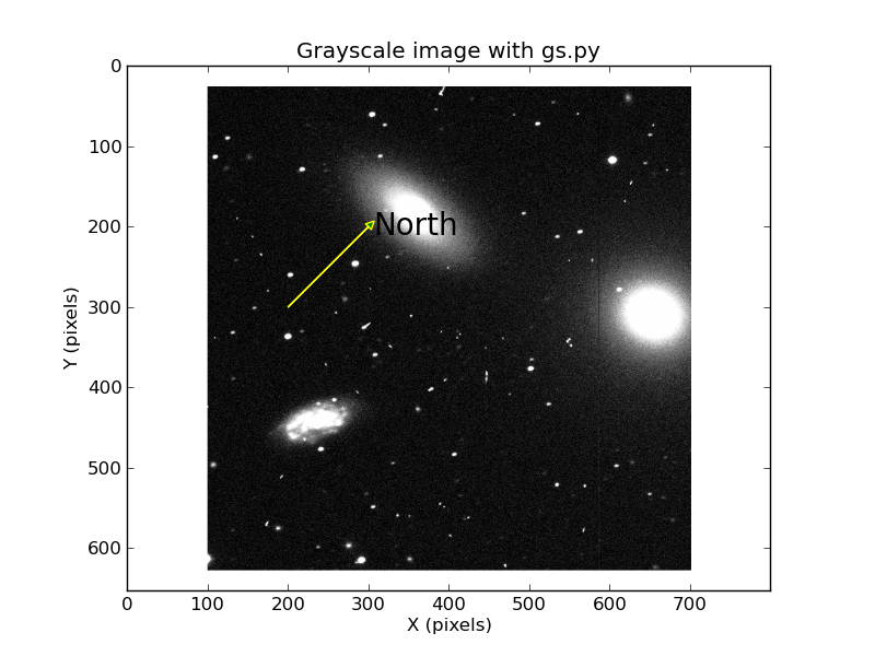Here is the type of image I can generate using a bone-head simple python script that utilized the matplotlib package. I've taken the png file from the above exercise and run the command: % gs.py c_sub_800_800.png Of course, the overplotted markers and text are nonsense and used here only as a demonstration. An important word of WARNING: if you are a good ds9-er, you'll know that normally the image will be displayed with +X pixels going to the right, and +Y pixels going to towards the top of the display. This is the way our pixel coordinates will be read in our very top NGC3379 graphic above. Notice that the configuration of stars and galaxies around NGC3379 (the round galaxy) is the same in all of our images. However, the Y-axis pixels are labeled above in our python version with +Y values increasing towrads the bottom. We'll have to be mindful of such things when creating things like finding charts, etc.. with packages like matplotlib. Some information on how gs.py works in this imshow tutorial.

1. I have a number coded that create the basic types of plot information: the IHMP outline (ihmp.sh), the VIRUS IFU pattern (vir_ifu_pat.sh), the outline of the HET guide probe annulus (het_gp_pickle.sh). The basic XY data sets made with these tools are in units of arcseconds, and have an origin at 0,0. I generally refere to these as APERTURE files.
2. The job of preparing aperture APERTURE file for a particular image involves a scale change, rotation, and translation. These produce files with X,Y in pixel units, and they are typified by codes like cbf_trans.sh (closed boundary files, for the IHMP), lsegs_trans.sh (line segments, e.g. for IFU bounds or guide probe annuli), text_trans.sh (for marking text, e.g. for labeling IFU names).
3. The actual preparation of the ds9 region files is done with python scripts (.../codes/python/ds9 ) like: xyr_circles_ds9.py, lines_file_ds9.py, lsegs_file_ds9.py, text_file_ds9.py. Some of these routines take parameters on the command line and produce a region string, some take the name of a fle and produce strings for multiple regions.

IMPORTANT VIRUS TOOL NOTES: I had a lot of notes on routines I developed to overplot VIRUS and HET features on DSS (and other ) images. These notes, and support run scripts are all in:

 
 Test_Data_for_Codes/T_runs/Image_Render/ex0_n3379/S 

The ImageMagic routines (mostly convert) can be used to perform a many simple (and not so simple) image-processing tasks. I would never trust this stuff to process images for science purposes, but it sure is handy sometimes to get things into cartoon-like state for building figures. Moreover, it seems to come intsalled with almost every linux distribution you can think of. Some discussions and Here are detailed ImageMagic examples are here. The bottom line to date is that I DO NOT UNDERSTAND much of the image processing tasks employed in the ImageMagic convert task. I spent the better part of an evening and morning reading web material, and it is clear that some important concepts elude me. I think the primary confusion has to do with the fact that the PNG and other standard rendering files assume 8-bit (2^8 ---> 0 to 256) pixel ranges. Moreover, a lot of the special transform features ("-fx") assume ranges of 0 to 1. What seems to be missing inthe online stuff (to me at least!) is any kind of reasonable explanations of how you take images with larger ranges (i.e. FITS images with BITPIX=-32 floating point pixels) and prep them to the point of using convert on them. So, I move on for now and investigate other routes to rendering astronomical images with a useful dynamic range.

Originally I envisioned a document here that just described how I "make an image" from something in a FITS file. That is clearly the overall goal, but I have found after my experience with ImageMagic, that some other capabilities of python may be put to very good use now. Specifically, viewing pixel histograms (standard and cummulative) will help me to understand the basics of image display. I can use the gs.py code described above in my introduction, but getting to the useful PNG file that this code needs is a bigger subject. In the following link I discuss image rendering using python. The real work is in establishing the transfer function that gets my FITS pixels into the 8-bit (0 to 256) range (for instance) that makes for a good PNG image.

A variety of tool sets have been combined to create a general-purpose rendering tool for VIRUS. The properties of this tool are described here.

I describe software tools used in the Nov2015 LRS2 commissioning run. This is meant to record some of the methodology used during early commissioning tests and does not imply anything about future observing procedures.