1. Visualizing the HET sky footprint.
2. Visualizing the guide probes.
3. Visualizing the ACAM footprint.
4. Locating an HET guide star.

The HET acquisition camera (ACAM) seems to be the primary means of confirming where the HET is pointed on the sky. After the HET is sent to a sky position (Ra,Dec) by the telescope control system (tcs), we general take an image with the ACAM to visualize where the etelescope is presently pointed. The TO is genearlly asked to manually move the HET such that a given sky position (Ra,Dec) falls on a specific position on the ACAM, usually a position referred to with a variety of names: boresite, IHMP center, w-axis. The idea here is that by placing a known sky position at a known location in the ACAM we are also positioning some other instrument. Examples of this are putting a science target on a VIRUS IFU or placing a bright guide star on a guide camera. It is very helpful when the RA/TO team has a means of visualizing these operations in real time.

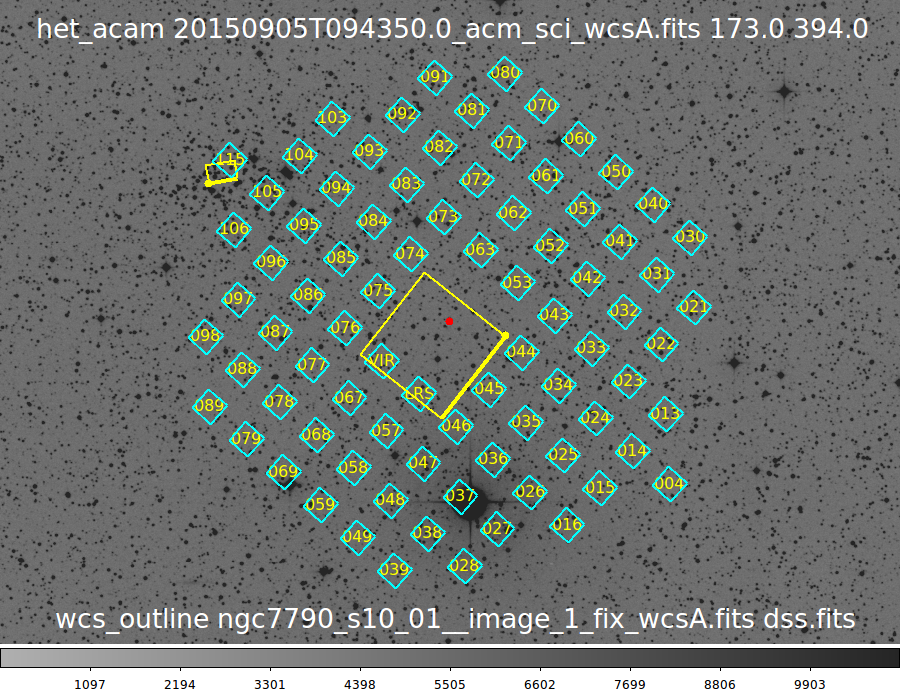Here we visualize the "sky footprint" of an HET pointing. We used two commands with two images. The two images were had WCS information installed in their FITS headers using software tools (e.g. wcs_doall) discussed elsewhere in these documents. The images were: 20150905T094350.0_acm_sci_wcsA.fits: The wcs-calibrated ACAM image. This is represented by the large yellow box in the picture above. ngc7790_s10_01__image_1_fix_wcsA.fits: A wcs-calibrated dsi10 image. In Aug2015 a number of small digital cameras were intalled in IFUSLOT positions on the IHMP. The small yellow box represents an image made with camera dsi10, which was installed in IFUSLOT 115 on the IHMP (IHMP = IFU Head Mounting Plate). Our picture shows a number of things that are critically important for the TO/RA to understand when setting up an observation with the HET. First, the small red dot shows the location of the IHMP on the sky. The small yellow dot at one corner of large yellow box represents ACAM pixel position X,Y=1,1, and the thick yellow line in the large box shows the Y=0 line (i.e. the first row of pixels) in the ACAM image. A similar box is made for the dsi10 image (in the upper-left). We also see the position of the VIRUS IFU array, including the Nov2015 positions of the LRS2 Red IFU (LRS) and the single VIRUS IFI (VIR). This figure was made with the two command shown at the top and the bottom of our picture: het_acam 20150905T094350.0_acm_sci_wcsA.fits 173.0 394.0 * This draws the HET sky footprint when the ACAM image named 20150905T094350.0_acm_sci_wcsA.fits was taken. The assumed IHMP center in ACAM pixel units was assumed to be (X,Y)_ihmp = 173,394. wcs_outline ngc7790_s10_01__image_1_fix_wcsA.fits dss.fits * This draws the outline of our wcs-calibrated dsi10 image. The name of that image was ngc7790_s10_01__image_1_fix_wcsA.fits, and the second arguments on the command line (dss.fits) was the name of the FITS image we actually display with ds9 for the view of the sky field above.

% got 
% cd ./T_runs/het_acam/ex0_n7790
% S/grab 

For this HET pointing:    Ra,Dec,AZ = 23:57:23.975 +61:07:37.37 336

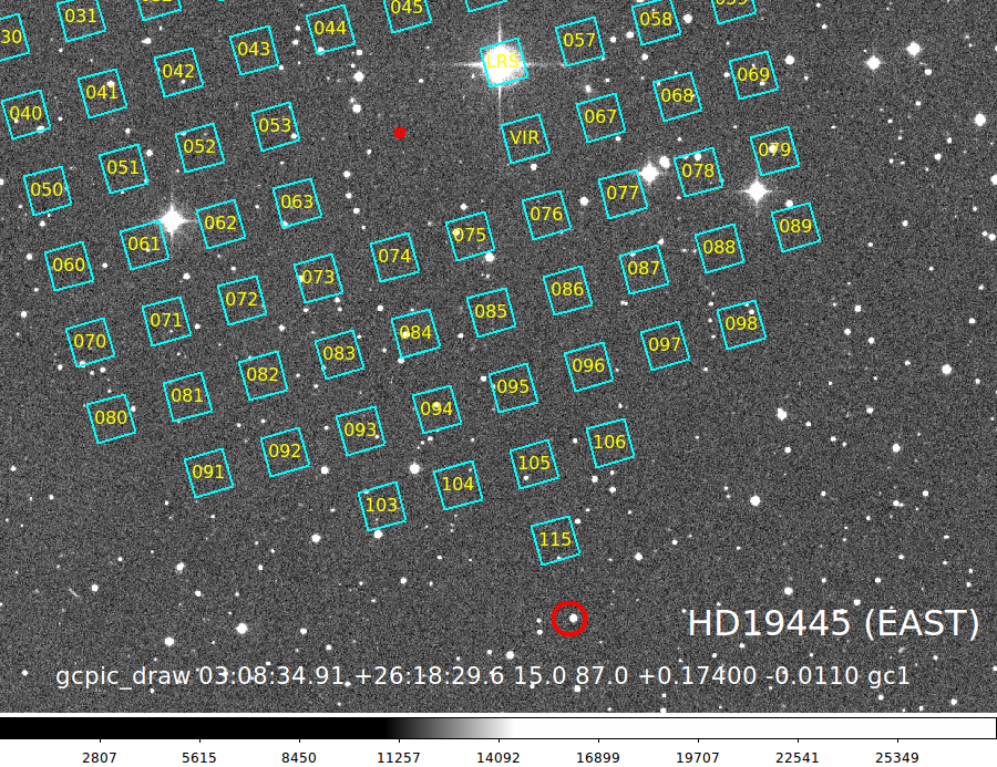Pointing for the EAST track of HD19445. The flux standard HD19445 was a target for LRS2 commisioning tests, as well as testing the positioning of the guide probes (in the case below we consider Guide Probe 1 = gc1). gcpic_draw 03:08:34.91 +26:18:29.6 15.0 87.0 +0.17400 -0.0110 gc1 Y The primary goal in this pointing was to place HD19445 in the LRS2 IFUSLOT position. This fixes the position of the IHMP (used above). In the case of the guide star, I have adjusted gc1 from the initial X-axis location (Telecen X,Y = +0.15996 0.0000) so that a relatively bright star falls into the gc1 field (X,Y = +0.17400 -0.0110). The >font color=red>large red circle above shows the predicted position of gc1. By adjusting the values of the input Telecen X,Y values (arguments 5 and 6 on the command line) we are able to place a bright guide star candidate into the gc1 field of view. Strategy: We have no bright star at the IHMP (boresite) location. There are one or two nearby faint stars that "bracket" this position, so I would suggest we use the ACAM images to APPROXIMATELY position the IHMP center at RA,DEC = 03:08:34.91 +26:18:29.6.

The het_acam example discussed above, but what good is it if you happen to not have a WCS-calibrated ACAM image. This is the more common case. Suppose we have a position on the sky (Ra,Dec in J2000) and the structure azimuth (AZ) that we'll use to observe with? For instance, let's use the Ra,Dec,AZ values from the het_acam example above (Ra,Dec,AZ = 23:57:23.975 +61:07:37.37 336).

 
 acam_fake 23:57:23.97 +61:07:37.4 336.0 178 391 Y  

Usage: acam_fake 23:57:24.01 +61:07:35.8 336.0 178.0 391.0 Y
arg1 - RA  (sexigecimal)
arg2 - DEC (sexigecimal)
arg3 - Azimuth of HET structure (degrees)
arg4 - X_ihmp 
arg5 - Y_ihmp 
arg6 - Display with ds9 (Y/N) 
Note for ihmp: X,Y= 173 394; later X,Y= 178 391 

To make the image WITHOUT displaying it with ds9:
 acam_fake 23:57:23.97 +61:07:37.4 336.0 178 391 N  
 
Our ACAM image should have at X,Y=178,391
a sky position of Ra,Dec(J2000) = 23:57:23.840 +61:07:37.27

% xy2sky acam_dss.fits 178 391
23:57:23.965 +61:07:37.40 J2000 178.000   391.000     (Good) 

To paint the "fake" acam outline:
wcs_outline acam_dss.fits dss.fits 

To paint the field with gcpic_draw:
% gcpic_draw 23:57:24.01 +61:07:35.8 15.0 336.0 -0.031 -0.134 gc1 Y

 
% acam_fake 23:57:23.97 +61:07:37.4 336.0 178 391 N
% ds9_open 1000 1000 
% xpaset -p ds9 file dss.fits                       
% xpaset -p ds9 scale limits 0.0 20000.0
% xpaset -p ds9 zoom to fit  
% wcs_outline acam_dss.fits dss.fits             

The modules discussed above can now be used to rather easily locate suitable stars for the HET guide probes. Basically, we make an initial run of gcpic_draw to paint up the field. Next, we select a star that is near (or far from!) our GC red circle marker. We establish the X,Y of that desired star in the corrdinate system of our display image (dss.fits). Using these coordinates, and a step size in degree units, we use the routine named gcpic_grid" to derive the x_ang,y_ang (lately called Telecen_X, Telecen_Y) for the guide probe of interest. Using a second gcpic_draw run with these x_ang,y_ang values, we have our final finder chart. Moreover, gcpic_draw now gives us "fake" acam image for the pointing (with WCS and pixels painted using the DSS images) that is displayed as a yellow outline. With this (FITS) image the TO can set up accurately on the field.

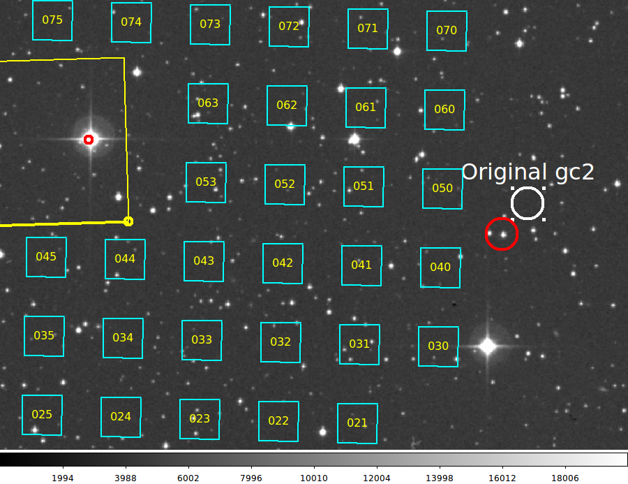Here is the final product of a gcpic_draw run that shows a well-selected guide star for gc2 (Guide Probe 2). The commands used were: % gcpic_draw 03:37:40.75 +38:25:47.0 15.0 294.0 -0.018 0.153 gc2 Y % gcpic_grid 0.025 1531.7 894.7 % gcpic_draw 03:37:40.75 +38:25:47.0 15.0 294.0 -0.029 0.144 gc2 Y The gcpic_draw arguments are explained in the figures above (also see below in this caption). By interactively viewing the first gcpic_draw run, I was able to quickly choose a bright star near the gc2 probe at a position in the DSS image frame (the image displayed) of X,Y=1531.7 894.7 (and this position I used to run gcpic_grid). The gcpic_grid arguments are the step size in degree units for the search grid, and the X,Y position (in dss.fits pixel units) of the star we desire to use as a guide star. For completeness I also show the tcs command we would use to move the gc2 probe for this position: guider@htcs% syscmd -T -v 'Guider2_set_position( x_ang=-0.029000, y_ang=+0.144000) ' guider@htcs% syscmd -T -v 'pfip_move_probes()' It should be noted that as of late Nov2015, the yellow outline of the "fake" acam image is now painted into every rendering made with gcpic_draw. The small red circle indicates the position of the IHMP center projected to the sky, and the larger red circle shows the sky-projected position of the guide probe (in our case here that would be gc2). In the figure above, I have added (in white) the original position of gc2 that was displayed when we first ran gcpic_draw. The red gc2 circle above is that resulting from our second run of gcpic_draw where we have used the x_ang,y_ang values were predicted by the gcpic_grid run. As you can see, we have repositioned gc2 so that it now contains a bright guide star for this pointing (i.e. for this projection of the focal plane on the sky). For completeness, here are the usage messages for the gcpic_ commands (as of Dec2, 2015): To render a finding chart Usage: gcpic_draw 21:53:53.89 +62:36:52.6 15.0 342.0 -0.031 -0.134 gc1 Y Usage: gcpic_draw 23:57:24.01 +61:07:35.8 15.0 336.0 +0.15444 -0.00111 gc1 Y arg1 - RA (sexigecimal) arg2 - DEC (sexigecimal) arg3 - faintest USNO RED magnitude arg4 - Azimuth of HET structure (degrees) arg5 - x_ang of probe (degrees) arg6 - y_ang of probe (degrees) arg7 - probe name arg8 - open a ds9 window (Y/N) To derive x_ang,y_ang for a desired guide star Usage: gcpic_grid 0.015 618.0 1343.0 arg1 - grid spacing in degrees arg2 - desired X in DSS pixels arg3 - desired Y in DSS pixels