Here I explore some image display and computation methods using python.

1. The stinkbug.
2. Starting with the matplotlib tutorial.
3. Adding things and filling in gaps.

The peculiar name of this section derives from the title of a sample image (stinkbug.png) that I found in a matplotlib tutorial on how to use the imshow() task to make image plot. I downloaded the PNG file stinkbug.png and stored it in my TDATA location. Because the file is very small (unlike my FITS files), I decided to store it in the run diretory:

 
% got
% cd T_runs/Image_Render/ex1_stinker/S
% ls
stinkbug.png

 
% gs.py stinkbug.png
% display gs.png
% identify stinkbug.png
stinkbug.png PNG 500x375 500x375+0+0 8-bit DirectClass 108KB 0.000u 0:00.000
% display stinkbug.png

Finally, I since stinkbug is small, I decided to put a copy of it in my python code directory. This is where I began the simple gs.py code in python/implots (IMage PLOTS). I will leave gs.py alone, but I'll start building plot codes with stinkbug, and then work up to making image plots with the other image file there named n3379_B.png (the I made manually using ds9). Some other interesting points I learned as I read the page presenting stinkbug.png is:

1. Color PNG images are usually referrrd to as RGB or RGBA (where the A referes to a transparency channel).
2. grey scale images are just one channel
3. the PNG is called 24-bit becasue it uses THREE 8-bit images: one each for R, G, B.

 
% stink1.py stinkbug.png
Input file: stinkbug.png
Type for image is type 'instance'
Type for arr is type 'numpy.ndarray'

Use to view your plot:
display stink.png

I followed the matplotlib tutorial on the imshow module to build the code on codes/python/implots/stink2/stink2.py. I added a few lines to make some axis labels and create an output plot file.

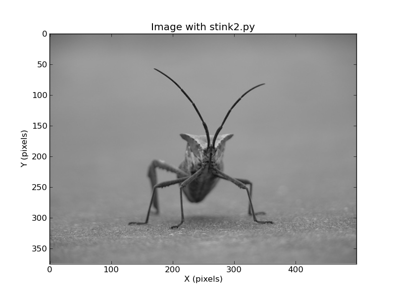The image made with stinkbug.png using stink2.py. The code is simple, but I show it here as a record of something that worked. #!/usr/bin/python # # Here I implement things from matplotlib tutorial at # http://matplotlib.org/users/image_tutorial.html # # To run: stink2.py stinkbug.png from sys import argv script_name, pngname = argv import matplotlib.pyplot as plt import matplotlib.image as mpimg import numpy as np # read the image file img=mpimg.imread(pngname) # Make the image plot imgplot = plt.imshow(img) # label the axes label_main = "Image with stink2.py" label_xaxis = "X (pixels)" label_yaxis = "Y (pixels)" plt.title(label_main) plt.xlabel(label_xaxis) plt.ylabel(label_yaxis) plt.savefig('stink.png') print '\nUse to view your plot:\ndisplay stink.png\n'

Here we start to fill in more things. I create a single-channel numpy array and plot it with a color lookup table. After some searching around, I found the names of the available lookup tables. As shown below, I make a new color table, but also I add a colorbar for that table. Perhaps the most important thing to notice is that (somehow) my pixel values are now in the range 0 to 1.

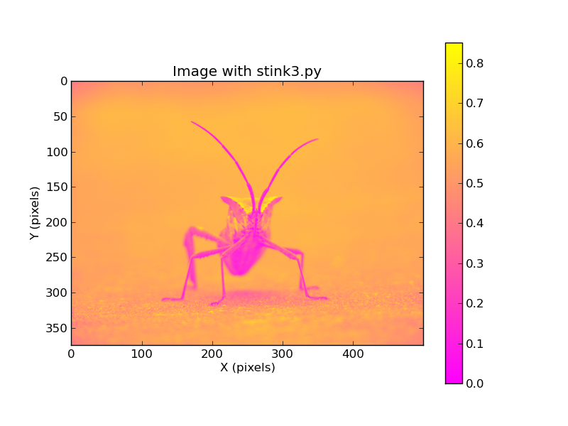The image made with stinkbug.png using stink3.py. The important thing to know here is that I changed the pixel scale to 0-1, and the code that did this is: # read the image file img=mpimg.imread(pngname) # Now build a numpy array lum_img = img[:,:,0] print "Type for lum_img = %s" % (type(lum_img)) # lum_img is a single channel image (the B part of RGB?) As usual, this important step is glossed over in the tutorial, but this appears to have involved something called "array slicing".