A more detailed discussion of trs_apply
The trs_apply routine combines all of the low-level trs_ transformation routines to
create a single script that uses one input parameter file tp perform an X,Y transformation.
- A simple run of trs_apply.
- The input parameter file.
- A collection of trs_apply sample runs.
A simple run of trs_apply.
Let's take our second exmaple of test data in our
discussion of trs_make_xy_TestData and
use trs_apply to transform those coordinates. We'll plot the original X,Y set, then
the transformed set.
 |
Here is a simple trs_apply example. We aim to take the point at X,Y=500,500
and translate (shift) it to the position X,Y=450,490.
# We make the test data file (file1.xy):
% cat t.1
500 500
500 600
700 500
450 450
% trs_make_xy_TestData read
% trs_plot.py Style.file 200 800 200 800 SHOW (optional)
% cp XY0.data file1.xy
# Notice that point 1 is at X,Y=500,500.
% cat TRS.1
500.0 500.0 N 1.0 0.0 0.0 0.0
# XoS YoS flip scal theta XoF YoF
# So, you can guess that I am just doing a translation here!
# Transform the XY, write no header, write to standard out
% trs_apply file1.xy TRS.1 N
0.000 0.000
0.000 100.000
200.000 0.000
-50.000 -50.000
# Transform the XY, write a header, direct the data to a file (file2.xy)
% trs_apply file1.xy TRS.1 Y > file2.xy
% cat file2.xy
# data
# data
0.000 0.000
0.000 100.000
200.000 0.000
-50.000 -50.000
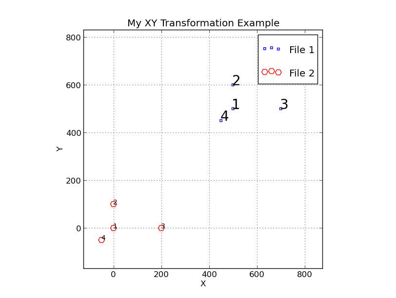
# Plot the file1.xy and file2.xy data in one plot
% trs_2plot file1.xy file2.xy "My XY Transformation Example"
% trs_plot.py Style.file 0 1000 0 1000 SHOW
Notice that we have indeed translated Point 1 (originally at X,Y=500,500) to
the new position at X,Y=0.0.
|
Notice tat in the example above I used an specialized plotting tool named
trs_2plot to build my input files for running trs_plot.py. Maybe a second
example using a primitive (but pervasive in the codes!) tool would be useful. This
tool, named "trs_build_plot_file" is easy to use. It will take as input the
name of your XY data file (e.g. file1.xy). You'll also specify a few arguments
that set the properties of the points (type, size, color) and a text string that
describes this set. I direct this output to a file (e.g. XY2.plot) and I can add
this file to the local "Style.file". When I run trs_plot.py this second (transformed)
data set is included. The advantage here over trs_2plot is that we could build a plot
with as many XY data files as we wish. In the figure below I give an example similar
to the obe above, but I use this more general approach to making the plot.
 |
Here is another simple trs_apply example. We aim to flip the points about the X axis.
% ls
file1.xy PointNames
% cat TRS.2
500.0 500.0 N 1.0 0.0 -450.0 -490.0
# XoS YoS flip scal theta XoF YoF
# So, you can guess that I am performing two translations here!
# Transform the XY, write a header, direct the data to a file (file2.xy)
% trs_apply file1.xy TRS.2 Y > file2.xy
% cat file2.xy
# data
450.000 490.000
450.000 590.000
650.000 490.000
400.000 440.000
# Build a plot file for the file1.xy data
% trs_build_plot_file file1.xy r s 100 25 "Original set" > XY1.plot
# Green (g) hexagon points (h) of size 140 with labels of size 25
% cat XY1.plot
point r s 100 25
Original set
500 500 1
500 600 2
700 500 3
450 450 4
# Build a plot file for the file2.xy data
% trs_build_plot_file file2.xy g h 140 25 "Translated set" > XY2.plot
# Green (g) hexagon points (h) of size 140 with labels of size 25
% cat XY2.plot
point g h 140 25
Reflected set
450.000 490.000 1
450.000 590.000 2
650.000 490.000 3
400.000 440.000 4
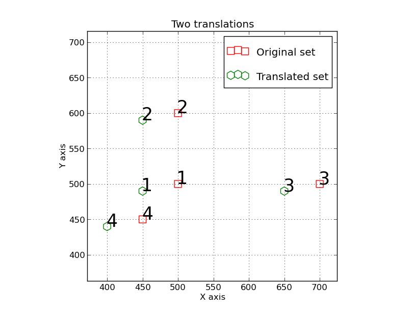
I edit or compose Style.file:
% cat Style.file
Two translations
X axis
Y axis
XY1.plot
XY2.plot
% trs_plot.py Style.file -1000 1000 -1000 1000 SHOW
Notice that I use a wider range of axis limits.
We sse that we have tranformed the Point 1 at X,Y=500,500 to be
at X,Y=450,490. By changing the last two arguments in the TRS file we have
applied a second translation that determined a new origin for our final
transformed set (in file2.xy).
|
The input parameter file.
A way to produce a set of random X,Y data points is described here.
To apply all of the coordinate transformation steps:
% trs_apply
Usage: trs_apply file1.xy trs_terms Y
arg1 - file with XY to be transformed
arg2 - file with TRS terms
arg3 - output header line (Y/N)
Terms: XoS YoS Reflect(X,Y,N) scale theta XoF YoF
XoS,YoS = X,Y to set origin in original system
XoF,YoF = X,Y to set origin in final system

An example of the "file with TRS terms":
% cat TRS.terms
    0.0    0.0     Y      1.0   0.0     0.0  0.0
#   XoS    YoS    flip    scal  theta   XoF   YoF

The tranformed X,Y are sent to standard out, but general redirected to some new file.

% trs_plot.py Style.file -30 30 -30 30 SHOW
Hence, the first pair of coordinates (XoS,YoS) establish the new origin for the
initial (input) set of coordinates. After the reflection, scale, and rotation
operations are performed, the second pair of coordinates (XoS,YoS) establish the
origin in the final (output) set of coordinates.
A collection of trs_apply sample runs.
A set of trs_apply examples are given now to give us a sense of how each parameter
in the TRS input file change the output X,Y values. I build a script named
trs_apply_demoscript.
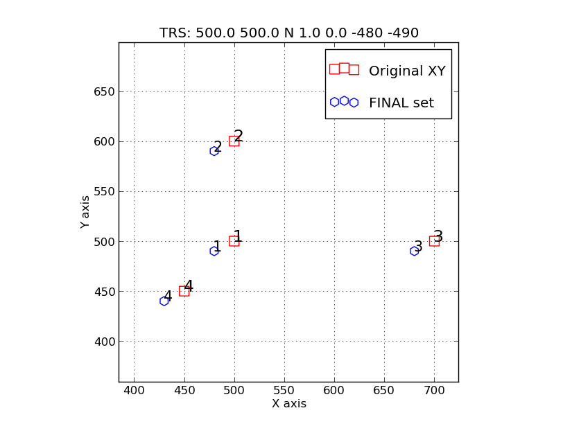 |
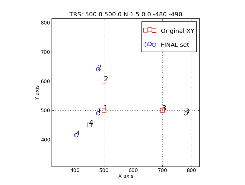
Example 1: Two transalations have been used to shift the transformed points
(blue) to the left and down relative to the original (red) points. The
full sequence of transformations performed by trs_apply (seen in
trs_apply_ex.STEPS) is shown here:
   Step1:   trs_translate.sh file1.xy 500.0 500.0
   Step2:   trs_reflect.sh xy.step1_translate N
   Step3:   trs_scale.sh xy.step2_reflect 1.0
   Step4:   trs_rotate.sh xy.step3_scale 0.0
   Step5:   trs_translate.sh xy.step4_rotate -480 -490
|
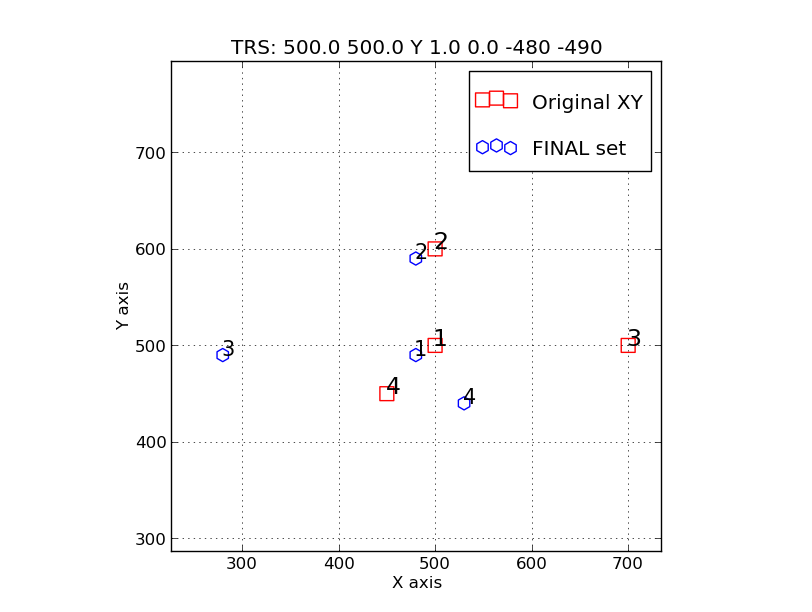 |
Example 2: In addition to the translations of example 1 above, we
have now reflected (flipped) the points about the Y axis (specified by
argumen 3 in the TRS file). Note that the reflection was performed with:
trs_reflect.sh xy.step1_translate Y
|
 |
Example 3: In addition to the translations of example 1, we
have now applied a scale change of Sfactor=1.5.
Note that the scale adjustment was performed with:
trs_scale.sh xy.step2_reflect 1.5
|
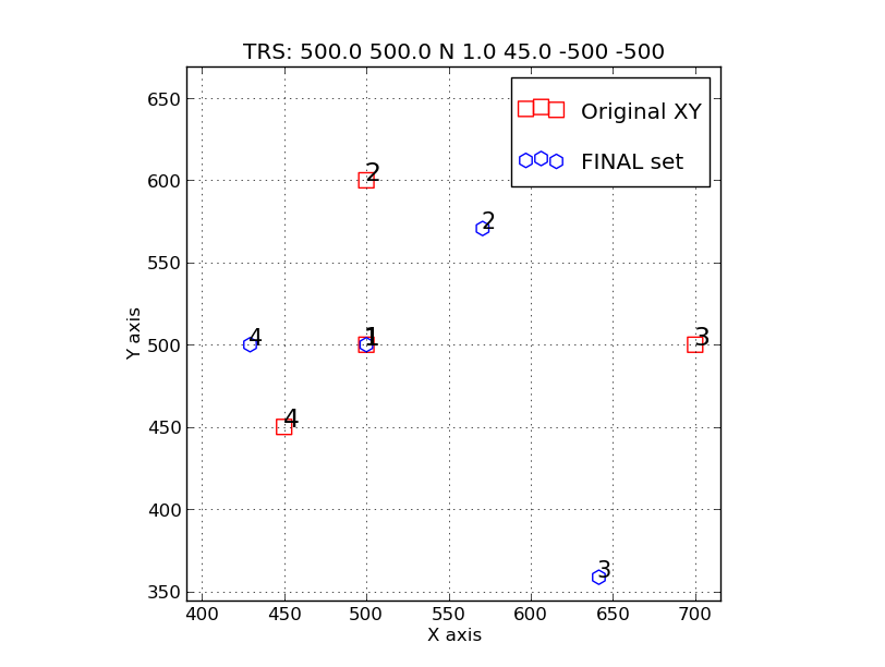 |
Example 4: Here we see an example of a rotation by 45 degress.
To make the sense of thr rotation more evident I dispensed with
the translation. Hence, the point of rotation (Point 1) remains
fixed in the transformed set. A positive rotation angle in degree units
(theta) produces a CLOCKWISE (CW) rotation by trs_apply.
Note that the rotation was performed with:
trs_rotate.sh xy.step3_scale 45.0
|
Back to calling page