Generate a data using a function in one dimension. Note that a higher level script named make_fit_data uses this routine, along with some others, to generate curve data with added noise. Some useful initial commands for gen_curve.sh are:

% gen_curve.sh
Usage: gen_curve.sh line coefs.1 50 1.0 10.0
arg1 - type of curve (L for list)
arg2 - name of coefficients file
arg3 - number of points
arg4 - xmin 
arg5 - xmax 
arg6 - header flag (Y/N) 

% gen_curve.sh L # Generate a listingof available functions  

Helpful Note:  
This routine requires thet the input coefficients file (e.g. coefs.1) be present. 
The routine make_fit_data allows the user to construct this file "on the fly". You 
can do this manually: 

Usage: make_coeffs_file poly4 file.1 
arg1 - type of curve 
arg2 - name of coefficients file to be created 
Examples: 
  % make_coeffs_file poly3 c.1 
  % make_coeffs_file r4sph coeffs.spheroid 

1. Generate and plot a parabola.
2. Generate a noisy parabola.
3. A good collection of fancier examples.

To generate a polynomial using 3 terms and then make a quick plot I show the following figure:

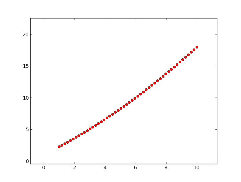To generate a parabola I use the following run gen_curve.sh with the input file c.3. Notice that since I'll be using 3 terms in the polynomial equation to generate the data, the type of function (the first argument to gen_curve.sh") will be "poly3". My input file that contains the values of the terms (one value per line) can be named anything ("c.3 in this example). % cat c.3 1.0 1.2 0.05 % gen_curve.sh poly3 c.3 50 1.0 10.0 N > MyData % ipython In [1]: from scomods.ascii_tools import * In [3]: x=read1col("1","MyData") In [4]: y=read1col("2","MyData") In [5]: import matplotlib.pyplot as plt In [6]: plt.plot(x,y,"ro") In [7]: plt.show() In [9]: quit() Note that the I used the matplotlib show() routine to manually adjust the scale and placement of the the final X,Y axes before I generated the plot file above. This is a handy way to quickly view data. I have made use of my own ASCII reading tool in the above example. See my document on using ipython for more explanations and examples. Note also that in this example I used arg6=N, so no header file preceded the generated curve data. In this case the header was written to a local file named "gen_curve.explain".

Here I use the oned_imarith.sh routine to add noise to a test curve.

To generate the noiseless parabola:
% gen_curve.sh poly3 c.3 50 1.0 10.0 > MyData.1 

To generate noise:
% gen_noise.sh gaus 50 0.0 2.0 > noise.1 

To add noise to MyData.1:
% oned_imarith.sh MyData.1 + noise.1 MyData.2 

RECALL: You can add randomness to the generated noise by adding a seed file:
% date > seed 

During Summer2016 I compile a lot notes on ipython, matplotlib and numpy. I had some good curve generating examples there. These notes were tucked away with the very descriptive title "bunch o notes". For safer keeping, I placed a copy of these nice curve examples here.