ds9_profiles
Updated: May16,2020 This code is obsolete. A revised version is ds9_profiles_x

Interactively generate and measure profiles in an image using a ds9 gui. It should be stressed that this is a test bed code to aid in developing image analysis methods. It is not meant for efficient batch-processing of numerous targets on an image. Rather, I use this to create a variety of diagnistic statistics and graphics that clarify and validate procedures like background estimation, profile extraction, and photometric parameter (e.g. R50) estimation.


% ds9_profiles --help 

# A typical call to ds9_profiles 
% ds9_profiles Rsco2039.fits default default none N

This code was begun in Oct2015, and was substantially revised in Oct2018. It has a dedicated matplotlib plot package, but much of the Oct2018 work was dedicated to creating a set of uniformly produced table files (*.table and *.parlab) that can be use to make a variety of plots with table-oriented codes like xyplotter_auto. Later I created dedicate packages for plotting profiles like clip_margdist_sub_plotter and profile_plotter.

Sample data and exercises.

Supporting routines.

Sample data and exercises.

You can access some sample images packed into a tarball VIA THIS LINK. Below I show how I pacjed the tarball, how I can unpack it, and a brief description of the images.

 

% tar cvzf TestData.tar.gz Test_ds9_profiles # How I packed the data  
% tar xvzf TestData.tar.gz # How I would unpack the data  

The test images in ./Test_ds9_profiles/images:

Rsco2039.fits  == R PFC image of the NGC3379 field. The imag is wcs- and zp-calibrated. 
  Useful for testing the ellipse and circle region use.

20181111T032020.1_056RL_flt.fits == bias subtracted LRS2 Qth image (flat lamp). 
  Useful for testing the box (horizontal) region use. 
  The OBJECT name for this image is "Qth_R",  where the R indicates this was taken 
  through the red light guide.  This test image was made with: 
  lrs2_bias_sub.sh /home/sco/LRS2_Nov15_Tests/Data_1/20181111T032020.1_056RL_flt.fits

20181115T044859.1_056RL_cmp.fits == bias subtracted LRS2  (arc lamp) 
  Useful for testing the box (vertical) region use. 
  The OBJECT name for this image is "Hg_R",  where the R indicates this was taken 
  through the red light guide.  This test image was made with: 
  lrs2_bias_sub.sh /home/sco/LRS2_Nov15_Tests/Data_1/20181115T044859.1_056RL_cmp.fits

20180403T075403.4_acm_sci_proc.fits == a typical acm image with a few stars. The image 
   was processed (ACM_reduced_gcprobes_Sep2018/) with a rough fixed bias pattern correction 
   and a wcs solution was installed in the header.

I will periodically add sample exercises to the list below.

Supporting routines.

A number of routines were developed for ds9_profiles. I briefly review the most useful routines below.

 
 # make radius image = pixels give radius within region  
% ellradius.sh
arg1 - X dimension of output image
arg2 - Y dimension of output image
arg3 - X center in pixels 
arg4 - Y center in pixels 
arg5 - circle radius (asemi) in pixels 
arg6 - axis ratio (b/a) 
arg7 - PA in degrees (GALPHOT convention)

# Collect the profile points for a region using the radius image 
% profile_pnts.sh
arg1 - name of fits image to be measured
arg2 - name of (fits) radius image (from ellradius.sh)
arg3 - sky value (fits image or fixed-number)
arg4 - pixel mask (can be "none")
arg5 - run in debug/verbose mode
# creates useful file:   profile_pnts.table,parlab 

# Compute the growth curve 
% profile_gcurve.sh
Usage: profile_gcurve.sh profile_pnts.out 20.0 N 
arg1 - name of input text file (profile_pnts.out)
arg2 - Maximum radius in pixel units
arg3 - run in debug/verbose mode 
# creates useful file:   profile_gcurve.table,parlab  profile_gcurve_kfit.table,parlab  

# Build a plot file  
% profile_plot_01.py -h
usage: profile_plot_01.py [-h] [-v] arg1 arg2 arg3 arg4 arg5
positional arguments:
  arg1           input data file
  arg2           low value for X axis
  arg3           high value for X axis
  arg4           low value for Y axis
  arg5           high value for Y axis
optional arguments:
  -h, --help     show this help message and exit
  -v, --verbose  Verbose responses
# creates useful file: As of Oct26,2018 user can opt for hardcopy with show()

The type of plot made with profile_plot_01.py may change, but an example from Oct26,2018 is shown below. The description in the figure caption should remain generally useful.

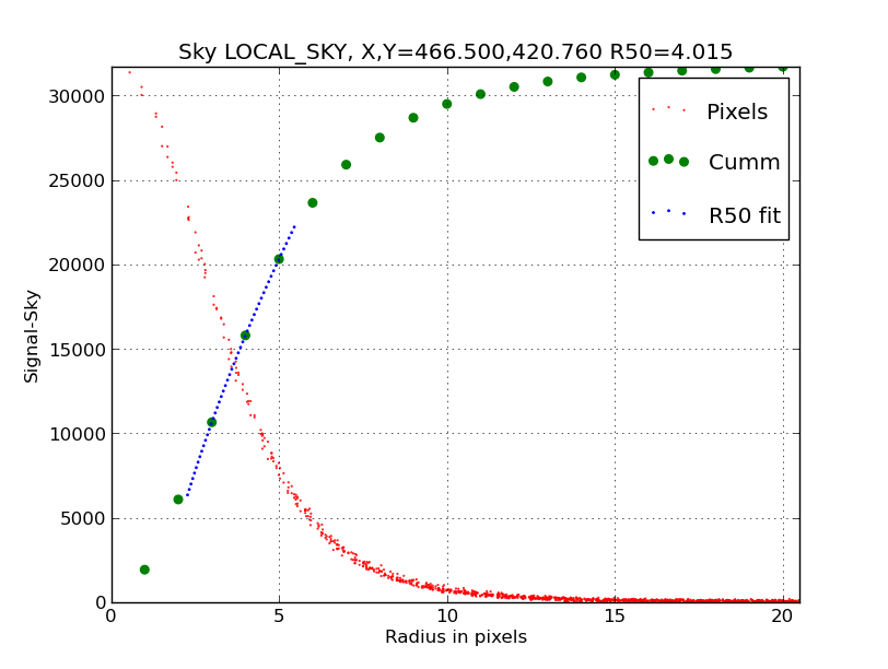
A simple radial profile of a star measures on a 20180403 acm image. The small red points are values from individual pixels collected with the profile_pnts.sh routine, which uses a FITS image map of the target radius balues (from ellradius.sh). Integration of this raw "profile" is performed with profile_gcurve.sh, and the growth curve (also known as the cummuuative distribution) from this code is plotted above as green circles. The small blue points represent a polynomial ft to a section of the growth curve around k=0.5 for the purpose of estimating R50 (the "half-light" radius).

NEW FEATURE (Nov25,2018):

The profile data and plot files are archived to local subdirectories with the name ap_*, where * is the region line number. The code used for this is: ds9_profile_archive


Usage: 
  ds9_profile_archive 1 box N
  ds9_profile_archive 2 ellipse N

Back