- Initial Observing Notes
- A quick survey of the acm image sets
- A master set of acm targets.
- Measuring the acm image sets.
- Measuring the gc1 image sets.
- Measuring the gc2 image sets.
- Plate scales are measured and plotted.
Initial Observing Notes
On 20190724 we (SCO/NM) made observations designed for deriving the gc1,gc2 plate scale. We
took sets of acm,gc1,gc2 images with guiding done on acm. We moved the acm fiducial to
to perform the telescope offsets. We used about 7 offsets, with the last two done with
no "pid loop".
Original notes made by SCO:
==================================================================================

20190724
A: SCO   TO: NM
===========================================================
ENG    gc offset test to derive plate scale

Moon is about 20deg above horizon, and 60% illum

target_setup 54 E -cat gp -ifu 000
This field: 54    GALl110bm5  23:18:39.51  +55:31:29.69     2000  34.3  15.00 06:51 02:11 07:49 01:55

To make acm offsets:
   syscmd -T 'ACQ_offset_fiducial ( dx_asec=5,dy_asec=0,compensate="false")'

Go to target at 06:55 UT
Note DIMM seeing is jumping to 2" just as we get going on this test!

Position START
Starting set of 10 at 07:02:22 UT    (stars centered in gc1,gc2)
Stop taking images at at 07:04:32

Position A
At 7:05
   syscmd -T 'ACQ_offset_fiducial ( dx_asec=5,dy_asec=0,compensate="false")'
*** star moves straight down on gc2
wait for focus and guider stability
Start taking images at   07:08:06 UT
stop 07:10:21

Position B
At 7:10:52
   syscmd -T 'ACQ_offset_fiducial ( dx_asec=-10,dy_asec=0,compensate="false")'
star moves over, but stys well within gc1,gc2
wait for focus and guider stability
Start taking images at   07:14:24 UT
stop 07:16:53

Position C
At 7:17:10
   syscmd -T 'ACQ_offset_fiducial ( dx_asec=+5,dy_asec=-6,compensate="false")'
wait for focus and guider stability
Start taking images at   07:20:30 UT
stop at 07:22:47

Position D
At 07:23:20
   syscmd -T 'ACQ_offset_fiducial ( dx_asec=0,dy_asec=+12,compensate="false")'
   syscmd -T 'ACQ_offset_fiducial ( dx_asec=0,dy_asec=+2,compensate="false")'
wait for focus and guider stability
Start taking images at   07:30:15 UT
stop at 07:32:29

Position E
At 07:33:25
   syscmd -T 'ACQ_offset_fiducial ( dx_asec=0,dy_asec=-14,compensate="false")'
wait for focus and guider stability
Start taking images at   07:37:00 UT
stop at 07:39:20

DIMM is hopping up to 2" again

With pid set to ZERO
Position F  (same as E, but pid is off)
wait for focus and guider stability
Start taking images at   07:41:00 UT
stop at 07:43:33

Position G
At 07::43:54   (pid still off)
   syscmd -T 'ACQ_offset_fiducial ( dx_asec=0,dy_asec=+14,compensate="false")'
Start taking images at   07:45:55 UT
stop  07:48:30

Done with test
===========================================================

**** Thu Jul 25 14:00:54 CDT 2019
I have moved the 20190724 acm,gc1,gc2 full data sets to:
/media/sco/DataDisk1/sco/AD/HET_work/acm_nights/20190724
(I have also move this to the steveo laptop)

The galpoint field (gp) I used for this is at:   23:18:39.51  +55:31:29.69
Recall that "galpoint" fileds are a list of low galactic latitude fields that
are listed in the htopx "gp" catalog. They are fields we use when we want a
hight number of stars in the field.
To get support data:
 % dssbase 23:18:39.51  +55:31:29.69  6.0 19.5 N
For a non-internet reduction I can use:   /home/sco/DSS_Base/acm_fields/Store_DSS

Here is a summary of the positions and their time intervals.
Position Set      Recorded UT Interval
------------    -----------------------
  START         07:02:22.0   07:04:32.0
  A             07:08:06.0   07:10:21.0
  B             07:14:24.0   07:16:53.0
  C             07:20:30.0   07:22:47.0
  D             07:30:15.0   07:32:29.0
  E             07:37:00.0   07:39:20.0
  F             07:41:00.0   07:43:33.0
  G             07:45:55.0   07:48:30.0
==================================================================================
A quick survey of the acm images for the night
You can read about how how I reviewed the images in each position/time interval
in a discussionn of processing acm images.
Here I want to review each set of acm images and delete images that show large
position departures. I then use the final image listing to establish a new
time interval for each position. The basic recipe is:
I perform this in:   /home/sco/GC_Plate_Scales/20190724

To get the initial catalog with image types:
  acm_table_markII N


  select_pas_images_by_time ACMDAT.images ACMDAT 07:02:22 07:04:32 STARTacm N
  bigds9 STARTacm.images 1 20
  mkdir STARTacm
  mv ds9_list_load.nomark STARTacm/list.0

  select_pas_images_by_time ACMDAT.images ACMDAT 07:08:06.0 07:10:21.0 Aacm N
  bigds9 Aacm.images 1 20
  mkdir Aacm
  mv ds9_list_load.nomark Aacm/list.0

  select_pas_images_by_time ACMDAT.images ACMDAT 07:14:24.0 07:16:53.0 Bacm N
  bigds9 Bacm.images 1 20
  mkdir Bacm
  mv ds9_list_load.nomark Bacm/list.0

  select_pas_images_by_time ACMDAT.images ACMDAT 07:20:30.0 07:22:47.0 Cacm N
  bigds9 Cacm.images 1 20
  mkdir Cacm
  mv ds9_list_load.nomark Cacm/list.0

  select_pas_images_by_time ACMDAT.images ACMDAT 07:30:15.0 07:32:29.0 Dacm N
  bigds9 Dacm.images 1 20
  mkdir Dacm
  mv ds9_list_load.nomark Dacm/list.0

  select_pas_images_by_time ACMDAT.images ACMDAT 07:37:00.0 07:39:20.0 Eacm N
  bigds9 Eacm.images 1 20
  mkdir Eacm
  mv ds9_list_load.nomark Eacm/list.0

  select_pas_images_by_time ACMDAT.images ACMDAT 07:41:00.0 07:43:33.0 Facm N
  bigds9 Facm.images 1 20
  mkdir Facm
  mv ds9_list_load.nomark Facm/list.0

  select_pas_images_by_time ACMDAT.images ACMDAT 07:45:55.0 07:48:30.0 Gacm N
  bigds9 Gacm.images 1 20
  mkdir Gacm
  mv ds9_list_load.nomark Gacm/list.0
I reject (mark) images with large motions indicated and then rename the list of
unamrked image to an appropriate name. I create a subdirectory with this image file
and record the final range of UT times. These final UT time intervals will be used
to gather the corresponding gc1 and gc2 image sets.
Here is a summary of the refined time intervals for each position.
Position Set      Refined UT Interval
------------    -----------------------
  START         07:02:39.7  07:04:18.3
  A             07:08:31.0  07:10:09.6
  B             07:14:50.5  07:16:43.1
  C             07:20:56.0  07:22:34.7
  D             07:30:32.0  07:32:24.7
  E             07:37:19.4  07:39:12.1
  F             07:41:18.4  07:43:25.0
  G             07:46:13.5  07:48:20.3
The above procedure is practical if we have only one or two position sets. In this
case we have 8 sets and performing all of these steps manually is laborous.
A BETTER and SAFE way to do this:
A better way to gather and visually review the images in each position set
is to use pas_time_window_sets.
Basically, I build one input file (along with the usual BaseDir and Date files) that
specieis each position name and time inetrval. For each set the names of images are
collected and run through bigds9, allowing
the user to reject bad images. Note that pas_time_window_sets is not specific to
acm images. Any type of PAS image can be treated. We'll use it to collect the
gc1 and gc2 images fro the corresponding positions. The code will form subdirectory
for each set where the cleaned image lists are stored. Finally, in each set
subdirectory the images are stacked to give a single image that represents the mean
field. Belwo I show how I processed the 8 positions for the acm images from 20190724.
% pwd
/home/sco/GC_Plate_Scales/20190724_red2
% ls
BaseDir  Date  S/  Time.Sets
% cat BaseDir
/media/sco/DataDisk1/sco/AD/HET_work/acm_nights
% cat Date
20190724
% cat Time.Sets
  START         07:02:22.0   07:04:32.0
  A             07:08:06.0   07:10:21.0
  B             07:14:24.0   07:16:53.0
  C             07:20:30.0   07:22:47.0
  D             07:30:15.0   07:32:29.0
  E             07:37:00.0   07:39:20.0
  F             07:41:00.0   07:43:33.0
  G             07:45:55.0   07:48:30.0

% pas_time_window_sets acm Time.Sets N
Note that as a sanity check I usually some in on a bright star and blink
the zoomed in image. When the set is completed, and I get the message like
"Set with name = A has been completed.", I manually record the X,Y position
of this star is eacj image set. I often find these rough positions useful in
verifying more precise offset calculations downstream in the reduction. I usually
just copy the Time.Sets file and fill in these XY values as I process each set.
  START         07:02:22.0   07:04:32.0     499.2  316.1
  A             07:08:06.0   07:10:21.0     500.6  298.0
  B             07:14:24.0   07:16:53.0     500.8  335.6
  C             07:20:30.0   07:22:47.0     478.6  315.0
  D             07:30:15.0   07:32:29.0     529.4  315.6
  E             07:37:00.0   07:39:20.0     475.8  316.9
  F             07:41:00.0   07:43:33.0     476.9  317.0
  G             07:45:55.0   07:48:30.0     530.0  315.8

NOTE:  Positions E and F appear to be the same! So, I could disregard F.

At the end of this run, my directory looks like:
% ls
Aacm/	       acmALL.params  acmALL.table  BaseDir  Dacm/  ds9_open.Size  Facm/  list.IMAGES  STARTacm/
acmALL.images  acmALL.parlab  Bacm/	    Cacm/    Date   Eacm/	   Gacm/  S/	       Time.Sets
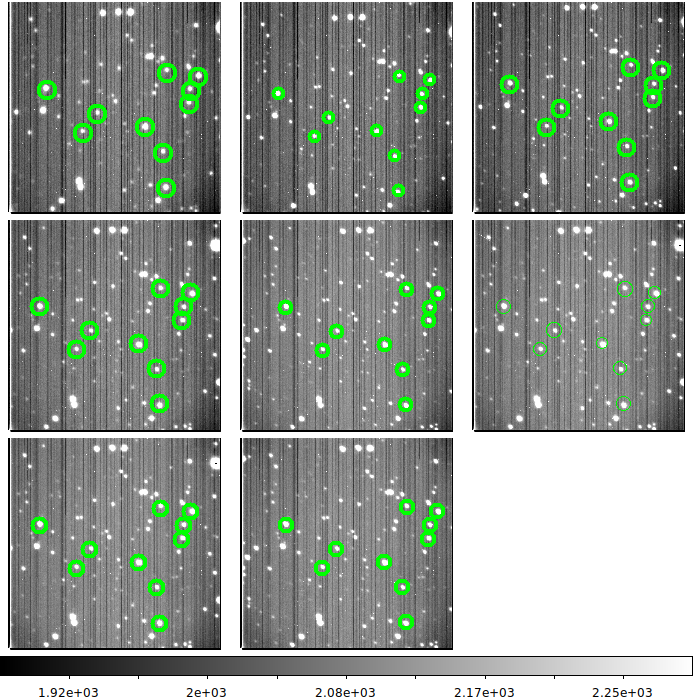
A master set of acm targets.
Typically I will also build a mosiac of the stacked fields and use the first image to
set up a set of acm stars that I will measure in each image set. For the subsequent sets
I use the ds9_region_xyshift.sh script
to apply XY shifts that will transform the XY coordinates of the original targets to
the coordinate system of each position set.
% pwd
/home/sco/GC_Plate_Scales/20190724_red2/figs_acm
% ls -1 ../*acm/*.fits >list.acm
**** I might edit list.acm *****
% bigds9 list.acm 1 10
***
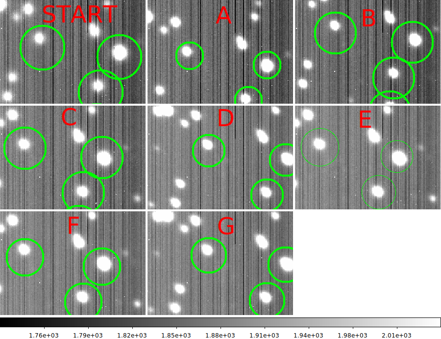
I blink the images to locate stars that do not leave the field
or get too close to the image edge to allow centroid calculation.
I save a set of regions for a good image, in this example I save: Eacm.reg
I note the FIRST object I marked in this chart. This is the object I will
identify in all subsequent images for which I'll to build a shifted region file.
Then I create shifted versions of Eacm.reg for each image:
% ds9_region_xyshift.sh ./Eacm.reg ../STARTacm/STARTacm.fits N
% ds9_region_xyshift.sh ./Eacm.reg ../Aacm/Aacm.fits N
% ds9_region_xyshift.sh ./Eacm.reg ../Bacm/Bacm.fits N
% ds9_region_xyshift.sh ./Eacm.reg ../Cacm/Cacm.fits N
% ds9_region_xyshift.sh ./Eacm.reg ../Dacm/Dacm.fits N
% ds9_region_xyshift.sh ./Eacm.reg ../Eacm/Eacm.fits N
% ds9_region_xyshift.sh ./Eacm.reg ../Facm/Facm.fits N
% ds9_region_xyshift.sh ./Eacm.reg ../Gacm/Gacm.fits N
At the end of this process I have the region files for each image:
Aacm.fits Bacm.reg Dacm.reg Eacm.fits Facm.reg list.acm STARTacm.reg
Aacm.reg Cacm.reg ds9_open.Size Eacm.reg Gacm.reg S/
Now I can rerun bigds9 and then manually load each region file in the
appropriate frame. I usually copy each region file to its appropriate
subdirectory (with a script).
% bigds9 list.acm 1 10
The two figures below illustrate this mosaic process with bigds9.
The position subdirectories gathered above now contain a list of images
(list.0), a mean stacked image of the field, and an appropriately shifted
region file. In the case of this reduction, each field will have the same
10 stars measured in each image of each position set. For each subdirectory
I would run command sequence like that below:
To measure position offsets
To compute the possible sets of offsets:
    cd /home/sco/GC_Plate_Scales/20190724_red2
    table_XY_offsets.sh ./Aacm/XYmean ./Bacm/XYmean xmean ymean xme yme N
    pas_XY_offsets.sh ./Aacm/list.0 ./Bacm/list.0 1.0  N

An easy script run:     ./S/ORUN Aacm Bacm
                        ./S/ORUN STARTacm Eacm
                        ./S/ORUN Cacm Dacm
                        ./S/ORUN Gacm Facm

Here I collect the acm position set offsets

           SCO centroid                                     PAS centroids                      Position Pair
     mean        median          m.e.  Nstar        mean         median        m.e.   Nims
     ---------------------------------------       ---------------------------------------
     35.719       35.959        0.293    10         37.156       37.256        0.519     8     A-B
     22.979       22.745        0.352    10         21.989       22.293        0.803     8     START-E
     52.101       52.203        0.112    10         52.159       52.421        0.454     8    C-D
     51.679       51.715        0.068    10         51.658       51.751        0.494    10    G-F
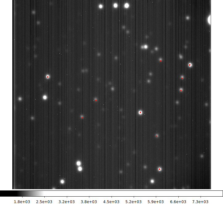
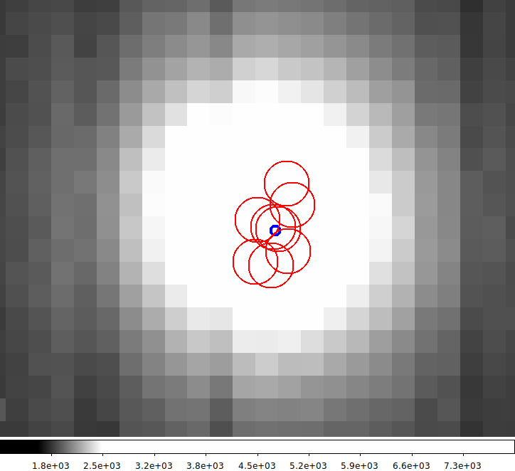
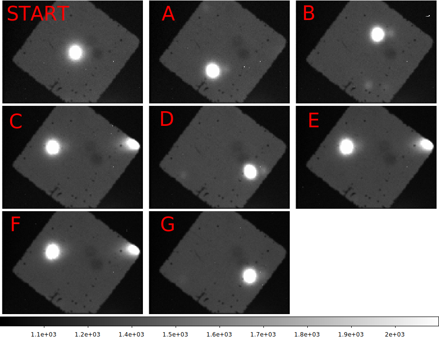
Measuring the gc1 image sets.
Because the gc images normally posess only a single bright star, the
mesaurement of the images is less complicated than the acm sets.
*** Gather the position set subdirectories ********
There are N=3423 gc1 images

% pwd
/home/sco/GC_Plate_Scales/20190724_red2
% ls
BaseDir  Date  S/  Time.Sets
% cat BaseDir
/media/sco/DataDisk1/sco/AD/HET_work/acm_nights
% cat Date
20190724
% cat Time.Sets_refined
  START         07:02:39.7  07:04:18.3
  A             07:08:31.0  07:10:09.6
  B             07:14:50.5  07:16:43.1
  C             07:20:56.0  07:22:34.7
  D             07:30:32.0  07:32:24.7
  E             07:37:19.4  07:39:12.1
  F             07:41:18.4  07:43:25.0
  G             07:46:13.5  07:48:20.3
% pas_time_window_sets gc1 Time.Sets_refined N

% pwd
/home/sco/GC_Plate_Scales/20190724_red2/figs_gc1
% ls -1 ../*gc1/*.fits >list.gc1
   **** I might edit list.acm *****
% bigds9 list.gc1 1 10

*** In each subdirectory for gc1
% ds9_imstats_fitslist list.0 FixedRegions N

To compute the possible sets of offsets:
    cd /home/sco/GC_Plate_Scales/20190724_red2
    table_XY_offsets.sh ./Agc1/XYmean ./Bgc1/XYmean xmean ymean xme yme N
    pas_XY_offsets.sh ./Agc1/list.0 ./Bgc1/list.0 1.0  N

An easy script run:     ./S/ORUN Agc1 Bgc1
                        ./S/ORUN STARTgc1 Egc1
                        ./S/ORUN Cgc1 Dgc1
                        ./S/ORUN Ggc1 Fgc1

Here I collect the acm position set offsets

           SCO centroid                                     PAS centroids                      Position Pair
     mean        median          m.e.  Nstar        mean         median        m.e.   Nims
     ---------------------------------------       ---------------------------------------
     51.748       51.748        0.403     1          51.296       51.381        0.532    20    A-B
     32.049       32.049        0.501     1          32.001       31.901        0.660    20    START-E
     71.346       71.346        0.421     1          71.235       71.287        0.466    19    C-D
     71.227       71.227        0.417     1          70.705       70.868        0.521    24    G-F
 |
|
The mean (stacked) gc1 images. The position set is indicated by the large red letters.
|
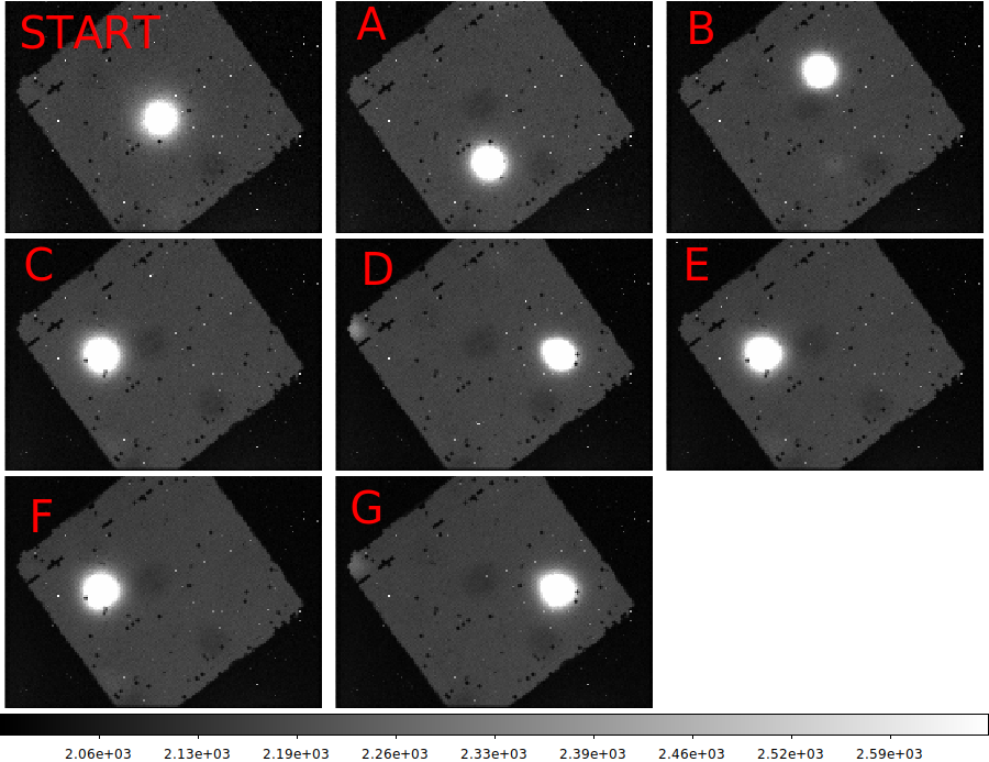
Measuring the gc2 image sets.
Here I present the same procedure for gc2.
*** Gather the position set subdirectories ********
There are N=3821 gc2 images

% pwd
/home/sco/GC_Plate_Scales/20190724_red2
% ls
BaseDir  Date  S/  Time.Sets
% cat BaseDir
/media/sco/DataDisk1/sco/AD/HET_work/acm_nights
% cat Date
20190724
% cat Time.Sets_refined
  START         07:02:39.7  07:04:18.3
  A             07:08:31.0  07:10:09.6
  B             07:14:50.5  07:16:43.1
  C             07:20:56.0  07:22:34.7
  D             07:30:32.0  07:32:24.7
  E             07:37:19.4  07:39:12.1
  F             07:41:18.4  07:43:25.0
  G             07:46:13.5  07:48:20.3
% pas_time_window_sets gc2 Time.Sets_refined N

% pwd
/home/sco/GC_Plate_Scales/20190724_red2/figs_gc2
% ls -1 ../*gc2/*.fits >list.gc2
   **** I might edit list.acm *****
% bigds9 list.gc2 1 10

*** In each subdirectory for gc1
% ds9_imstats_fitslist list.0 FixedRegions N

To compute the possible sets of offsets:
    cd /home/sco/GC_Plate_Scales/20190724_red2
    table_XY_offsets.sh ./Agc1/XYmean ./Bgc1/XYmean xmean ymean xme yme N
    pas_XY_offsets.sh ./Agc2/list.0 ./Bgc2/list.0 1.0  N

An easy script run:     ./S/ORUN Agc2 Bgc2
                        ./S/ORUN STARTgc2 Egc2
                        ./S/ORUN Cgc2 Dgc2
                        ./S/ORUN Ggc2 Fgc2

Here I collect the acm position set offsets

           SCO centroid                                     PAS centroids                      Position Pair
     mean        median          m.e.  Nstar        mean         median        m.e.   Nims
     ---------------------------------------       ---------------------------------------
     51.715       51.715        0.383     1        51.617       51.526        0.477    20      A-B
     33.071       33.071        0.498     1        32.604       32.629        0.627    20      START-E
     71.238       71.238        0.385     1        71.347       71.620        0.457    20      C-D
     71.079       71.079        0.398     1        71.171       71.451        0.520    24      G-F
 |
|
The mean (stacked) gc2 images. The position set is indicated by the large red letters.
|
Plate scales are measured and plotted.
The plate scale values for the offsets are computed.
I collect offsets in
% pwd
/home/sco/GC_Plate_Scales/20190724_red2/PS_extimates
Build a file names 20190724.dat:
% cat 20190724.dat
A-B
     35.719       35.959        0.293    10         37.156       37.256        0.519     8     A-B
     51.748       51.748        0.403     1          51.296       51.381        0.532    20    A-B
     51.715       51.715        0.383     1        51.617       51.526        0.477    20      A-B
START-E
     22.979       22.745        0.352    10         21.989       22.293        0.803     8     START-E
     32.049       32.049        0.501     1          32.001       31.901        0.660    20    START-E
     33.071       33.071        0.498     1        32.604       32.629        0.627    20      START-E
C-D
     52.101       52.203        0.112    10         52.159       52.421        0.454     8    C-D
     71.346       71.346        0.421     1          71.235       71.287        0.466    19    C-D
     71.238       71.238        0.385     1        71.347       71.620        0.457    20      C-D
G-F
     51.679       51.715        0.068    10         51.658       51.751        0.494    10    G-F
     71.227       71.227        0.417     1          70.705       70.868        0.521    24    G-F
     71.079       71.079        0.398     1        71.171       71.451        0.520    24      G-F

Next we compute the plate scale
% gcps.sh 20190724.dat N

To make a plot of the estimates (for example):
 % Generic_Points N
 % xyplotter_auto gc1_plate_scales q q 1 N
   (edit Axws.1 List.1)
 % xyplotter List.1 Axes.1 N

I add the plot data to my older 3 set analysis in: /home/sco/GC_Plate_Scales/4sets
  xyplotter xyplotter List.1 Axes.1 N
  xyplotter xyplotter List.2 Axes.2 N

Here are the stats for ALL data from stable nights:

GC1:
% cat gc1_stable.dat
0.1973
0.1989
0.1989
0.1870
0.1886
0.1942
0.1945
0.1978
0.1981
0.1966
0.1980
% calstats.py -v gc1_stable.dat
Simple stats for numbers in: gc1_stable.dat
Mean                     = 0.19545
Median                   = 0.19730
Standard deviation       = 0.00391
Minimum                  = 0.18700
Maximum                  = 0.19890
Number of values         = 11
Mean error of then mean  = 0.00124

GC2:
% cat gc2_stable.dat
0.1948
0.1971
0.1975
0.1871
0.1875
0.1882
0.1909
0.1981
0.1978
0.1970
0.1967
% calstats.py -v gc2_stable.dat
Simple stats for numbers in: gc2_stable.dat
Mean                     = 0.19388
Median                   = 0.19670
Standard deviation       = 0.00430
Minimum                  = 0.18710
Maximum                  = 0.19810
Number of values         = 11
Mean error of then mean  = 0.00136

Finally, I derive weighted mean stats for only the 3 stable nights:
% pwd
/home/sco/GC_Plate_Scales/4sets/Only_Stable_Nights

% table_stats.sh PS_gc1 ps pserr N
mean,median,sigma,m.e.,n:
      0.195445       0.197300       0.004103       0.001237     11
Weighted estimates (mean,sigma,m.e):
      0.196391       0.003855       0.001162

% table_stats.sh PS_gc2 ps pserr N
mean,median,sigma,m.e.,n:
      0.193882       0.196700       0.004506       0.001358     11
Weighted estimates (mean,sigma,m.e):
      0.195371       0.004015       0.001211

**** Here are the final data file I used for the above stats
% cat PS_gc1.table
PS values from stable data nights
   Pair    cam   meth    Sep      ps     m.e.    date
# data
    AB      gc1   sco   12.1    0.1973  0.0015   20190711
    AB      gc1   sco   10.2    0.1989  0.0012    20190720
    AB      gc1   pas   10.2    0.1989  0.0013    20190720
    AB      gc1   sco    9.7    0.1870  0.0015    20190724
    AB      gc1   pas    9.7    0.1886  0.0020    20190724
    STE     gc1   sco    6.2    0.1942  0.0030    20190724
    STE     gc1   pas    6.2    0.1945  0.0040    20190724
    CD      gc1   sco   14.1    0.1978  0.0012    20190724
    CD      gc1   pas   14.1    0.1981  0.0013    20190724
    GF      gc1   sco   14.0    0.1966  0.0012    20190724
    GF      gc1   pas   14.0    0.1980  0.0015    20190724

% cat PS_gc2.table
Stable night gc2 estimates
   Pair    cam   meth    Sep      ps     m.e.
# data
    AB      gc2   sco   12.1    0.1948  0.0016   20190711
    AB      gc2   sco   10.2    0.1971  0.0011   20190720
    AB      gc2   pas   10.2    0.1975  0.0013   20190720
    AB      gc2   sco    9.7    0.1871  0.0014   20190724
    AB      gc2   pas    9.7    0.1875  0.0017   20190724
    STE     gc2   sco    6.2    0.1882  0.0028   20190724
    STE     gc2   pas    6.2    0.1909  0.0037   20190724
    CD      gc2   sco   14.1    0.1981  0.0011   20190724
    CD      gc2   pas   14.1    0.1978  0.0013   20190724
    GF      gc2   sco   14.0    0.1970  0.0011   20190724
    GF      gc2   pas   14.0    0.1967  0.0014   20190724

The parlab files:
% cat PS_gc2.parlab
posp   Name of Position Pair
cam    GC camera name
meth   Method (Sco centroids or PAS)
sep    Star Separation in arcseconds
ps     plate scale (arcsec/pixel)
pserr  mean error of plate scale (arcsec/pixel)
date   Date of the Observations (UT)
The 11 "stable night" values are used to compute the mesn values in the titles of
the plots below.
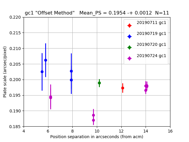 |
|
The gc1 plate scale from 4 nights of offset tests.
|
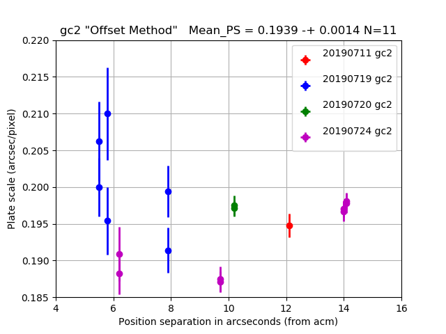 |
|
The gc2 plate scale from 4 nights of offset tests.
|
Back to calling page