The HET acquisition camera (acm) can be useful for a number of things. Here I
summarize some of the steps I use to process them. The term "process" is broad. This can be as simple
as how I detemine the types of images taken on a night or nights (how many bias or sky frames?). It
can concern how I correct the acm images for bias and dark signal. Other higher level steps like
deriving the WCS or photometric zeropoint calibrations and installing them in the image header were
established. In some cases, we may want to process a single image at a time, and if this is the case,
the reader should look at the web document for a routine named acmred.
The emphasis in this document is how we "process" an entire nights-worth of acm data.
Primary List
- Just the commands.
- Summarize multiple nights of acm data.
- Efficiently review a single night of acm images.
- Preparation for processing acm images.
- Processing acm images.
- Identify unique sky position image sets.
- Gather DSS and other calibration material.
- Compile catalogs of detected sources for each image.
- An appendix of older material.
Just the commands (Mar2020).
Here are the most current reduction steps.
  cd /home/sco/ACM_work_Oct2019/red_20191027
  AcmRunDate 20191027                                # Remember BaseDir file
  AcmRunDate_Clean Y


# View summary in the  file = ARD.Summary
Derive WCS for each onsky set and install WCS in image headers:

  isetwcs 1
  usno_look_wcs_fitslist isetwcs.images             # Optional review of image set
        usno_look_wcs_run blah.fits N               # For a super quick check


To get calibrated photometry for all sets:

   cat ./local_red/ISET_STACKS/list.* > List.1
   phot2_fitslist List.1 0.05 3


To review results (klunky):  gethead -u -f ./local_red/PHOT2/*.fits PSYSNAME ZPSEC ZPERR NUMZP SKYSB SKYSBERR VSKYSB  >phot2.20191022
To see "bad" images: cat Bad.List_phot
After these steps we have images with calibrated photometry. Various image propertues, including the night
sky surface brightess, are written to the FITS headers. These images are in the ./local_red/PHOT2 directory.
Return to top of page.
Summarize multiple nights of acm data.
To identify a useful night for acm image reductions, it is sometimes convenient
to to summarize lots of acm nights. You might want to know which nights have
bias frames take or lots of g images taken on the sky (i.e. image type = OPEN).
Here is a preocuder to do this.
% ls
BaseDir  list.dates
% cat BaseDir
/media/sco/DataDisk1/sco/AD/HET_work/acm_nights
% cat list.dates
20191018
20191020
20191022
20191026
20191027

% acm_nights_markII list.dates none N
% cat acm.nights_SUMMARY
Basepath used  = /media/sco/DataDisk1/sco/AD/HET_work/acm_nights

Number of nights to be surveyed  = 5

  Date       Ntot  Nopen Nbias Ndark Nnone Ntemps  NoB   Nog   Nor   Noi   Moon_illum
  20191018    587    355    20     0   202   587     0    99    23   232    84.100
  20191020   1003    323     5     0   665  1003     0   208     3   112    66.400
  20191022    722    609     5     0    98   722     0   437     0   172    44.900
  20191026    659    541     5     0   103   659     0   384     0   157     6.900
  20191027    422    361     5     0    46   422     0   240     0   121     2.100

Processing time for these nights = 26.000000 (seconds)

NOTE: To run Jan1,2017 to Sep11,2019 on mcs took a total of 5.7 hours.
One final thing to remember is that a single table file (basename=ALL) is compiled in
the above run. Information on every image from every surveyed night is compiled
in ALL. The ALL table from the Jan1,2017 to Sep11,2019 referred to above contained
over 200,000 images. You can use the point_selector code (as in the previous section)
to view these data. You can also view their associated images as long as you are
runiing on mcs. You can read more details about the OTW script
(acm_nights_markII).
Return to top of page.
Efficiently review a single night of acm images.
The most practical first step in evaluating a night of acm images is to compile a list
of the image names and their properties. By properties I mean things like image type
(bias,flat,dark,...), exposure time, filter name and so on. In additions, we'd like
to be able to easily view any of these images. The following commands enable this:
On sco2019:
% wheredata Y            # /media/sco/DataDisk1/sco/AD/HET_work/acm_nights,  20190724
% cat BaseDir
/media/sco/DataDisk1/sco/AD/HET_work/acm_nights
% cat Date
20190724
% acm_table_markII N
  10   0   455   54   (Nbias,Ndark,Nopen,Nnone)
% point_selector ACMDAT uthrs im N
The first command (wheredata) is just a short script that establishes
files (BaseDir and Date) that enable various routines to "know" the location of your image directory. The
following (acm_table_markII and
point_selector) are fairly high level routines that use multiple
codes. I have compiled more detailed descriptions and links about these.
Simply put, acm_table_markII gathers our image information into a data base (a "table file"), and point_selector
allows us to interactively view parameter spaces in this table file and easily view user-selected images with ds9.
Fianlly, it is worth noting here that the routine pas_imlistgen is
a key component to all of these routines. It is what gathers the initial list of images paths for the (BaseDir,Date)
you have provided. This script is for PAS images in general, not just the acm images.
As a benchmark, you should note that for the night of 20190724 we had a little over 500 acm images.
To run the acm_table_markII step on these images takes about 7 seconds on sco2019 and
about 26 seconds on mcs. The point_selector step, being an interactive graphics
routine is hard to compare in this way, but to be sure, most of the operations used in this routine
run much slower on mcs compared to sco2019 (or any newer machine). Finally, it may be of interest (but probably not)
to read some points concerning acm image handling.
Return to top of page.
Preparation for processing acm images.
The initial processing of an acm image inolves some FITS header repair, bias subtraction
(primarily FBP correction) and dark signal correction. By far, the most important step
here is the bias correction, and we use the following procedure to gather the bias data.
To get the bias data files for a night:
% acm_bias_for_date 20190207 N
    OR
% acm_bias_for_date none N
Note that the routine acm_bias_for_date will take the
date value from a local Date file if one is present, if not, it uses the value fed on the
command line. I configured it this way becasue soemtimes no bias images were taken on
a given date. We can use bias images from a few days before or after our night of interest.
Hence, we may want to delete the Date file and input our own date string for a night
when we know bias frames were taken. Another important point to remember is that for speed
purposes, if a "list.BIAS" file is present, then the images listed there are used as the
bias frames. This file (list.BIAS) is built in the initial run of
acm_table_markII, but if no bias frames were
taken for the night in question, then this file will be absent. In such a case, one can
run acm_table_markII for different nights until you get a list.BIAS file, and then you can
run acm_bias_for_date. Finally, note that
after this script has run, there are two new files present that will be used downstream:
BIAS.DATA  = contains the mean bias level and error
% cat BIAS.DATA
     1400.8599         0.8139
fbp.table   = contains the fixed bias pattern (FBP)
There will also be a local subdirectory (./bias) that contains a lot more information
about how the bias frames were stacjed and processed. Note that if you have no bias
frames, and you don't really care about accurate bias level subtraction (i.e. you are
not after surface brightness measurements), then you can always grab some bias files
with the following command:
% acm_get_bias N N
I have prepared a a general review of acm bias characteristics.
Return to top of page.
Processing acm images.
The routine that applies the bias (and other) data to the raw acm images
is paga. This name stands for "Process A Group of Acm".
% cat BaseDir
/media/sco/DataDisk1/sco/AD/HET_work/acm_nights
% cat Date
20190724
% acm_table_markII N
% acm_bias_for_date none N

% paga ACMDAT N
Usage: paga newacm N
arg1 - basename of table file (usually ACMDAT or newcam)
arg2 - run in debug/verbose mode
On sco2019, this run of 519 images took about 40 seconds to complete.
I keep some notes on paga performance.
Return to top of page.
Identify unique sky position image sets.
At this point, our processing steps have been computational inexpensive. Even on
on a slow machine like mcs a typical night of several hundred images can be processed in a
in a few minutes. However, in the following sections we'll encounter more complex
opertaions, some of which can involve user-interaction. The goal of this section is to
isolate a subset of only those images deemed useful for further reduction and for this I
developed a set of "onsky" routines.
I have early notes on developing the onsky routines.
After this step, we have a new table file with the target set numbers for
image sets that cover unique positions on the sky. The notes link describes various
files that can be used to graphically confirm the target field identifications.
The basic commands for this step, included in the recipe above, are
table_onsky_sets.sh and
onsky_set.
You can read more about the above example and see some illustrative figures
by following the onsky_set link.
Return to top of page.
Gather DSS and other calibration material.
For a lot of the processing discussed in this document we depend of
catalog data, prinmrily USNO-B1.0 and PS1 data sets. In many cases, a
standard DSS image that covers all or at least a portion of our acm
images can also be useful. Acquiring and then accessing this material
grew into its own document. You can read about
Gathering and using image calibration material.
Return to top of page.
Compile catalogs of detected sources for each image.
The image catalogs can be compiled in this section using
image_catalogs.
This routine uses a variety of object detection and sky mapping routines.
The user should note that the image parameters collected
these catalogs are based on intensity-weight momenst and isophotal
magnitudes. These are by no means "photometric" catalogs, but they are
quite adequate for establishing astrometric solutions for images in the
early stages of analysis.
% image_catalogs List.AllTargets TargetCats Y N

Usage: image_catalogs list.0 test Y N
arg1 - Name of file with list of input FITS images
arg2 - output directory name appendix (can be \|none")
arg3 - Clean all but the table files (Y/N)
arg4 - run in debug mode (Y/N)

I collected the full 536 acm images from 20190724 to do these timing tests
machine      S1     S2      S3       S4
sco2019     7sec    4sec   48sec    29min
Note that in the example above I used the list of target fields from the "onsky"
routines as input to image_catalogs. This
reduced the number of images to process from 587 to 76. Using the onsky images greatly
reduces our processing time.
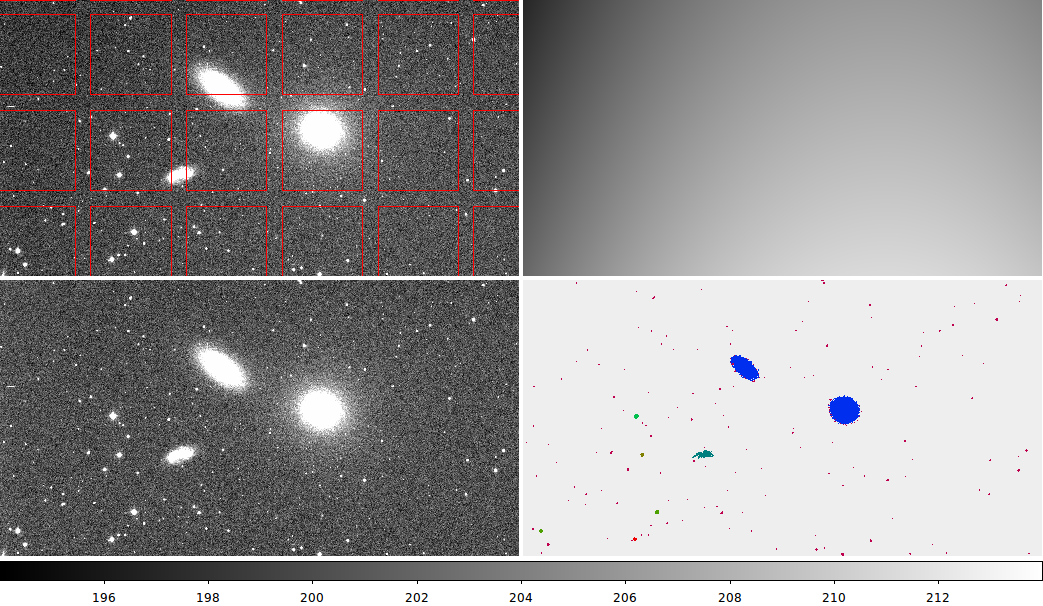
The basis for this catalog methodology is discussed in
Image Segmentation and
Contouring and is broadly summarized in the figure below.