Measuring telescope offsets on the sky can be used for a variety of problems. The basic tools behind how we measure the gc plate scales using offsets are shown below. Later I used some of these same tools to measure the offsets observed in dithered VIRUS observations. As I reduced more nights and tackled different problems, I began to compress and clarify the documentation. The basic results, ordered roughly by generality and clarity, are given below.

1. Measuring VIRUS fither offsets (Nov 2019)
2. Final report on gc plate scale measurements using offsets. (Oct 2019)
3. Early gc1,gc2 plate scale derivation studies. (Summer 2019) .

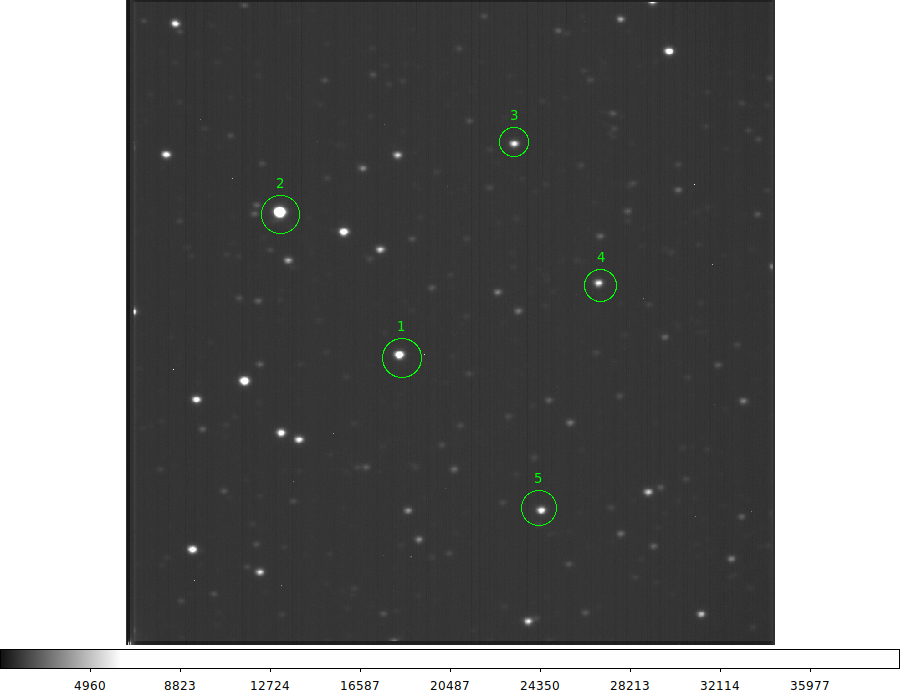
This is the last of a set of 12 acm images taken at one point on the sky, refereed to as PointA in this example. These images were collected during HET commissioning work after an FPA takedown on 20190711 (UT). I have marked 5, bright and fairly isolated stars. The stars are labeled so that we can measure the same set of stars (in the same order) at another sky position (PointB). The green circles represent the initial measurement apertures that will be used to derive an intensity-weighted centroid position for each star.

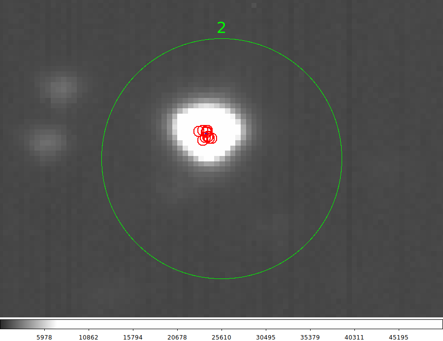This is a zoomed-in view of star 2 in the previous figure after the run of the measurement code (ds9_imstats_fitslist) has been run: % ds9_imstats_fitslist ./S/list.acm_A FixedRegions N The red circles represent the intensity-weighted centroid positions derived on each of the 12 images in the PointA set. Notice that the star image is slightly displaced from the center of the green "measuring aperture". This is becasue the green circle was set only approximately with a manually placed ds9 region (using the code ds9_imstats_markerII). The red circles do locate the star position on their respective images as they are derived from intensity-weight image centroids (i.e. first moments). The image displayed here is the last image in the set of set of 12 images made at PointA. The blue point is the mean position of the twleve centroids.

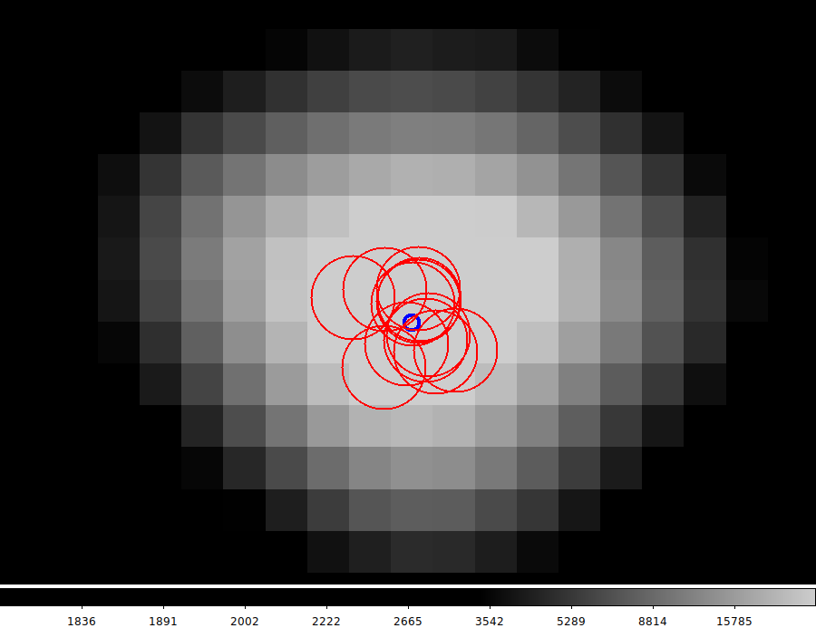
This is a "more zoomed-in" verison of the previous figure for star 2. Here we see he scatter of the image positions measured on each of the twelve PointA images (the red circles). Each red circle has a radius of 1 pixel. The thicker blue circle represents the mean position of these 12 centroids. The (blue) circle has a radius that is equal to the mean error of the mean X centroid posution (in pixel units).

The basic results from the two pointings (A and B) are tables of mean centroids for each of the 5 stars. Each table of mean value is named "XYmean", but they are written to different subdirectories and, hence, not overwritten. Note that for pointA we had 12 acm images, and for pointB we had 11 acm images.

What is each column of the table?  
% cat XYmean.parlab
xmean     Mean X centroid (pixels)  
xmedian   Median X centroid (pixels)  
xme       mean error of X centroid (pixels) 
nx        number of X positions  
ymean     Mean Y centroid (pixels)  
ymedian   Median Y centroid (pixels)  
yme       mean error of Y centroid (pixels) 
ny        number of Y positions  

For PointA: 
% pwd
/home/sco/GC_Plate_Scales/acm_A
% cat XYmean.table
# data
     326.21753      326.34000        0.17486     12	     347.81418      347.91998        0.18122     12
     183.01666      183.17499        0.18734     12	     518.46503      518.53497        0.19544     12
     463.34250      463.48001        0.17218     12	     600.42255      600.47998        0.18185     12
     564.21088      564.35498        0.17253     12	     433.29745      433.37500        0.17868     12
     495.47672      495.57501        0.17933     12	     161.39168      161.41501        0.16231     12

For PointB: 
% pwd
/home/sco/GC_Plate_Scales/acm_B
% cat XYmean.table
# data
     326.88727      326.92999        0.15816     11	     392.62180      392.76001        0.23252     11
     183.74182      183.66000        0.16528     11	     563.15729      563.31000        0.24223     11
     463.95450      463.94000        0.15841     11	     645.00092      645.15002        0.22412     11
     564.76733      564.79999        0.15992     11	     478.08545      478.17001        0.22294     11
     496.30820      496.34000        0.15377     11	     206.01181      206.00999        0.22103     11

The software used to perform the steps describe above are listed below:

ds9_imstats_fitslist ==  perform photometry on sets of images to derive tables files 
                         that contain XY centroids.  
Usage: ds9_imstats_fitslist list.in FixedRegions N  
arg1 - list of input images      
arg2 - case (none, FixedRegions) 
arg3 - run in debug/verbose mode 

table_XY_offsets.sh  ==  compile tables of mean offsets based on the table file from 
                         runs of ds9_imstats_fitslist. 
Usage: table_XY_offsets.sh tabA tabB XYmean xmean ymean xme yme N  
arg1 - basename of table 1 (A for A.table)    
arg2 - basename of table 2 (A for A.table)    
arg3 - param name for X position   
arg4 - param name for Y position   
arg5 - param name for error in X position   
arg6 - param name for error in Y position   
arg7 - run in verbose/debug mode (Y/N)

pas_XY_offsets.sh  == determine image offsets PAS X,Y centroids
Usage: pas_XY_offsets.sh list.1 list.2 N
arg1 - list of set1 PAS images
arg2 - list of set2 PAS images
arg3 - radius in pixels for the xy1,2.reg files
arg4 - run in verbose/debug mode (Y/N)

acm_offset == Given the acm offset (and error) in pixels compute the offset and
              error in arcseconds (for feeding to gcps.sh).
Usage: acm_offset 40.9708 2.1634
arg1 - offset in pixels
arg2 - mean error in pixels
arg3 - run in debug (Y/N)

gcps.sh  == compute gc plate scale when you know the acm offset and error in arcseconds
            and the gc offset in pixels
Usage: gcps Y
arg1 - run in debug mode