- Description of the Nov2019 dither test
- Pipeline processing of the acm images.
- Gathering images lists for the three dither positions.
- Stack images and make a master source list.
- Measure the master set targets in every image.
- Mean offsets with a single star.
- Mean offsets with multiple stars.
Description of the Nov2019 dither test
An set of engineering data was collected on 20191114. In this test we observed a
random field at a relatively low galactic latitude using the same dither procedure
used for VIRUS hetdex observations. Basically, after we execute the vlexp command to
take the dithered VIRUS data, we move the acm mirror into the system and takes acm
images for the duration of the dither sequence. I show the
vlexp command used to gather this data set, as well as the
Here are some useful summary notes and final table of useful times.
The field we used in f11 catalog:
target_setup 30989 E -cat f11 -ifu 000 -to

The vlexp command we ran:
vlexp -B -i virus -pobj Dither_Test -texp 20 -dither -np -vobs 7101 |& tee -a Adither.test

On my home machine (sco2019):
Data storage location:     /media/sco/DataDisk1/sco/AD/HET_work/acm_nights/20191114
Date reduction location:   /home/sco/Dither_Nov2019

What VIRUS "sees" is from the "Shutter Open" to "Shutter Closed" periods.
Hence, the three important times intervals are:
   P1     10:42:47.645  10:48:55.148
   P2     10:49:55.795  10:56:03.496
   P3     10:56:41.787  11:03:10.910
See the vlexp link given above for more details.
Return to top of page.
Pipeline processing of the acm images.
The acm images were processed with
a general acm pipeline . I used the pipleine only through the point of ccd_processing
the images and building a table file (ACMDAT) that I could view with point_selector.
% cat BaseDir
/media/sco/DataDisk1/sco/AD/HET_work/acm_nights
% cat Date
20191114

Steps I used:
% acm_table_markII N
% ./S/Get_Bias
% cp ACMDAT.images ACMDAT.images_raw
% paga ACMDAT N
% image_fullpath_list ACMDAT.images FIXUP newlist.images N
% mv newlist.images_version2 ACMDAT.images

I could view the images with:
% point_selector ACMDAT uthrs im N
# FBP subtraction not so great, but acceptable

To grab only the 150 images gathered for the entire vlexp sequence:
% select_pas_images_by_time ACMDAT.images ACMDAT 10:42:47.6 11:03:00.0 DALL N
% bigds9 DALL.images 1 200
In the last step above I could view all 150 images and blink them to observe
when the offsets occurred.
Return to top of page.
Gathering images lists for the three dither positions.
We now use the ACMDAT table and the 3 time intervals derived in the first section
to gather the sets of images for each dither position. I use a routine (select_pas_images_by_time)
to isolate the lists by time, then I review each set of images using the bigds9 routine. In this
latter routine I blink the images to identify any outliers. For our 3 sets below I found
no bad images and used the full set of 45 acm images for each point set. The final image lists and tables
are deposited in name-specific subdirectories.
*** All images in Point1
   P1     10:42:47.645  10:48:55.148
% select_pas_images_by_time ACMDAT.images ACMDAT 10:42:47.645  10:48:55.148 P1 N     # 45 images
% mkdir Point1
% cd Point1
% mv ../*P1* .
% ls
P1.images  P1.params  P1.parlab  P1.table
% bigds9 P1.images 1 100
% mv ds9_list_load.nomark P1final.images

*** All images in Point2
   P2     10:49:55.795  10:56:03.496
% select_pas_images_by_time ACMDAT.images ACMDAT 10:49:55.795 10:56:03.496 P2 N     # 45 images
% mkdir Point2
% cd Point2
% mv ../*P2* .
% ls
P2.images  P2.params  P2.parlab  P2.table
% bigds9 P2.images 1 100
% mv ds9_list_load.nomark P2final.images

*** All images in Point3
   P3     10:56:41.787  11:03:10.910
% select_pas_images_by_time ACMDAT.images ACMDAT 10:56:41.787 11:03:10.910 P3 N     # 48 images
% mkdir Point3
% cd Point3
% mv ../*P3* .
% ls
P3.images  P3.params  P3.parlab  P3.table
% bigds9 P3.images 1 100
% mv ds9_list_load.nomark P3final.images
At this stage I have three image lists, one for each vlexp dither position.
Return to top of page.
Stack images and make a master source list.
Now we want to stack the images at each pointing and establish a master list
of bright, well-isolated, stars in the stacked image field. We'll use the Point1
stack to identify the master set, then we'll use a routine that shifts this set
to the coordinate systems of the Point2 and Point3 sets.
For this we use ds9_region_xyshift.
% cd Point1/
% mkdir stack
% cd stack
% cp ../P1final.images .
% big_stack P1final.images 5 mean P1mean
% mv Big_Stack.fits P1mean.fits
% ds9 P1mean.fits                                 # I make the P1mean.reg file **************
% ls
P1final.images	P1mean.fits  P1mean.reg
% cp P1mean.reg ..

% cd Point2/
% mkdir stack
% cd stack
% cp ../P2final.images .
% big_stack P2final.images 5 mean P2mean
% mv Big_Stack.fits P2mean.fits
% cp ../../Point1/stack/*reg .
% ds9 P2mean.fits                                 # I do NOT save a regions file

% cd Point3/
% mkdir stack
% cd stack
% cp ../P3final.images .
% big_stack P3final.images 5 mean P3mean
% mv Big_Stack.fits P3mean.fits
% cp ../../Point1/stack/*reg .
% ds9 P3mean.fits                                 # I do NOT save a regions file
In the example above, we manually located stars in the field and save a ds9
regions file. In the other two mean image sets (for Point2 and Point3) we want to
display and measure the same stars. Beacuse the Point2 and Point3 images are
slightly shifted on the sky relative to Point1, we must derive and apply small
XY shifts to Point1 regions file.
For this we use ds9_region_xyshift.
To get the shifted region sets for P2 and P3 I use:
  Usage: ds9_region_xyshift.sh XYmean.reg a.fits N
  arg1 - Name of regions file to be shifted
  arg2 - Name of image defining new coordinate system
  arg3 - run in debug mode

P2:
% ls
P1mean.reg  P2final.images  P2mean.fits
% ds9_region_xyshift.sh P1mean.reg P2mean.fits N
% ls
P1mean.reg  P2final.images  P2mean.fits  P2mean.info  P2mean.reg
% cp P2mean.reg ..

P3:
% ls
P1mean.reg  P3final.images  P3mean.fits  S/
% ds9_region_xyshift.sh P1mean.reg P3mean.fits N
% ls
P1mean.reg  P3final.images  P3mean.fits  P3mean.info  P3mean.reg  S/
% cp P3mean.reg ..
Hence, at the end of this sequence of commands, we have region files in
each Point? subdirectory that identify the star we'll measure in each image set.
These stars will all be measures in the same order in each set.
Measure the master set targets in every image.
At this stage we have for each pointing (dither position) a list of images, and a ds9
regions file for a nicely selected set of stars in the filed. Each region file has
been adjusted to the coordinate systenm of each pointing.
For this we use ds9_imstats_fitslist.
Point1:
% ls
P1final.images	P1.images  P1mean.reg  P1.params  P1.parlab  P1.table  stack/
% ds9_imstats_fitslist P1final.images FixedRegions N
*** At the end I manually save the centroids markers in:   P1_centroids.reg
% ds9_region_circle2point XYcenStars.reg P1_XYcenStars.reg circle red N
% mv XYmean_me.reg P1_XYmean_me.reg
% mv XYmean_sig.reg P1_XYmean_sig.reg
% ls
local_red/	  P1final.images  P1mean.reg  P1.parlab  stack/		 XYmean.parlab	XYmean.table
P1_centroids.reg  P1.images	  P1.params   P1.table	 XYcenStars.reg  XYmean.reg

Point2:
% ls
ds9_open.Size  P2final.images  P2.images  P2mean.reg  P2.params  P2.parlab  P2.table  stack/
% ds9_imstats_fitslist P2final.images FixedRegions N
*** At the end I manually save the centroids markers in:   P2_centroids.reg
% ds9_region_circle2point XYcenStars.reg P2_XYcenStars.reg circle green N
% mv XYmean_me.reg P2_XYmean_me.reg
% mv XYmean_sig.reg P2_XYmean_sig.reg
% ls
ds9_open.Size  P2_centroids.reg  P2.images   P2.params	P2.table	   P2_XYmean.reg  XYcenStars.reg  XYmean.reg
local_red/     P2final.images	 P2mean.reg  P2.parlab	P2_XYcenStars.reg  stack/	  XYmean.parlab   XYmean.table

Point3:
% ls
ds9_open.Size  P3final.images  P3.images  P3mean.reg  P3.params  P3.parlab  P3.table  stack/
% ds9_imstats_fitslist P3final.images FixedRegions N
*** At the end I manually save the centroids markers in:   P3_centroids.reg
% ds9_region_circle2point XYcenStars.reg P1_XYcenStars.reg circle blue N
% mv XYmean_me.reg P3_XYmean_me.reg
% mv XYmean_sig.reg P3_XYmean_sig.reg
% ls
ds9_open.Size  P3_centroids.reg  P3.images   P3.params	P3.table	   P3_XYmean.reg  XYcenStars.reg  XYmean.reg
local_red/     P3final.images	 P3mean.reg  P3.parlab	P3_XYcenStars.reg  stack/	  XYmean.parlab   XYmean.table

As od Nov2019:
  I now produce two region files for the mean XY postions computed from all images:
     XYmean_me.reg    == the radius is the mean error of the mean
     XYmean_sig.reg   == the radius is the standard deviation about the mean
  Sometimes, with a lot of images, the latter can be very small.

  I modiied the ds9_imstats_fitslist file so that it displays BOTH of these mean region files.
Note that I have used ds9_region_circle2point
to make new marker files for showing the centroids of the individual stars from each image set. This
is because the regions files originally use circle marlers that have a radius of 1 pixel. This makes
for a crowded plot. Using point markers produces a better view for these dither sets.
Mean offsets with a single star.
I use a single star in the dither test set to make a figure and compute
mean dither offsets.
New dither figure with statistics (Fri Nov 22 13:30:12 CST 2019)
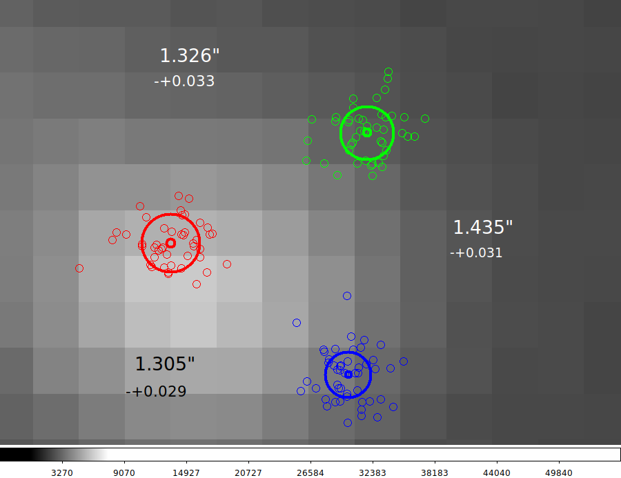
11 stars were measured in every image, but in the figure I show
a single star from a single image. The single image viewed here
is one from the the Point1 dither set. The mean dither positions
for this star, in acm pixel units, were found to be:
Point Color X (mean,m.e.) Y (mean,m.e.) Nimages
1 red 327.52 0.094 276.77 0.068 45
2 green 331.79 0.087 279.17 0.080 45
3 blue 331.38 0.073 273.89 0.083 48
Computing the mean offsets, and combining the mean errors in
quadrature, we derive the dither separations in units of pixels
and arcseconds (assuming ps_acm = 0.2709 -+0.0001 "/pixel)
for this single star:
Offset (pixels) Offset (arcsec)
sep m.e. sep m.e.
P1-P2 4.8983 0.12207 1.326 -+0.033
P2-P3 5.2959 0.11314 1.435 -+0.031
P3-P1 4.8160 0.10630 1.305 -+0.029
I have included these mean dither separations and their estimated
mean errors in the attached figure (zoom2.png).
Later today I'll compute mean offsets and errors using all 11 stars.
------------------------------------------------------------------
Scratch work
To get mean offsets and add mean errors qudrature:
For P1-P2
xyoff.sh 327.52 276.77 331.79 279.17
quadadd.sh 0.10 0.07 N
For P2-P3
xyoff.sh 331.79 279.17 331.38 273.89
quadadd.sh 0.08 0.08 N
For P3-P1
xyoff.sh 331.38 273.89 327.52 276.77
quadadd.sh 0.08 0.07 N
For conversion to arcsec assumin acm plate scale of ps = 0.2709 -+0.0001
fpmath.sh 4.8983 m 0.2709
fpmath.sh 0.12207 m 0.2709
fpmath.sh 5.2959 m 0.2709
fpmath.sh 0.11314 m 0.2709
fpmath.sh 4.8160 m 0.2709
fpmath.sh 0.10630 m 0.2709
P3-P1 4.8160 0.10630
To achieve better estimates of the dither offsets, we combine results from multiple
stars in the field. I have measured 11 stars in every image in eavery point set. The information
(gathered by the ds9_imstats_fitslist runs) is stored in the ./local_red/INFO subdirecties in
each of the Point subdirectories. More relevant to our task now, we have table files of
the mean positions for each of the 11 stars:
I revised the offset routine to give information on dX,dY. The new Results table is below