Offset Data Analysis to derive gc1,gc2 plate scales
Last Updated: Aug 26, 2019
Two methods were used to determine the plate scale (ps) in units of arcseconds/pixel for
the two guide probe cameras known as gc1 and gc2. Primary results and method descriptions can be
found in the firt two sections of this report.
Below I summarize the results from six nights of tests, giving weighted mean plate scale values
and error estimates for each guide probe camera. Next, I give a simple overview of a method
used to measure the plate scales of the HET gc1 and gc2 guide probe cameras. Four of the
nights had data collected using this offset method. Two of the
nights provided gc1,gc2 images that had multiple stars in their fields enabling a direct
solution of the world coordinate system (WCS) and hence plate scale. Following the initial
two sections I cover some of the details about how the data were observed and reduced.
Plots of the final sets of plate scales are shown.
- Summary of the results from 6 nights
- Overview of the offset method
- Observing notes
- A quick survey of the acm image sets
- A master set of acm targets.
- Measuring the acm image sets.
- Measuring the gc1 image sets.
- Measuring the gc2 image sets.
- Plate scales are measured.
- Final weighted mean values.
Summary of the results from 6 nights
The offset method was used on 5 different nights, with 3 of the nights providing
marginal data, and one of the nights (20190724) providing excellent data. The four
usable nights are summarized below.
    Night     Nacm,Ngc1,Ngc2    Offsets Done     Comments
   --------   --------------    ------------    ------------------------------------------------
   20190711     11,15,15             1          Usable, one offset
   20190719      8,27,17             2          Cloudy, bad image quality, No stabilization
   20190720     18,26,25             1          Very good stabilization
   20190724      9,19,19             7          Very good stabilization , many offsets
   20190712        NA               NA          Direct WCS measures by SJ of multi-star gc images
   20190713        NA               NA          Direct WCS measures by SJ of multi-star gc images

   Nacm,Ngc1,Ngc2 = Average number of (acm,gc1,gc2) images taken at each sky position
   Offsets Done   = Number of offsets performed to provide images at different sky positions
I received independent gc plate scale measurements from direct WCS solutions made by
Steven Janowiecki (SJ) in early July2019. I have added these results (2 fields
on two different nights) to the plots below (the "SJ" cyan points) and have added them
as independent measurements in computing the final weighted mean values and errors.
Tables of the best plate scale measurements and estimated errors for the gc1,gc2 plate
scales are given in the last section of this report. The final
weighted mean plate scale measurements are:
             Weighted Mean,error       Unweighted Mean,error    Number of points
             -------------------       ---------------------    ----------------
    GC1       0.1960   0.0009            0.1953   0.0009               15
    GC2       0.1953   0.0011            0.1943   0.0013               13
 |
|
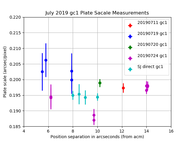
The gc1 plate scales from 4 nights of offset tests. I have also
added direct WCS gc1 measurements made by SJ in early July2019.
Note that the offset data of 20190719 were taken incorrectly (no
allowance for guiding stabilization). I include them for comparison, but
this night was rejected from the mean plate scale values reported here.
|
 |
|
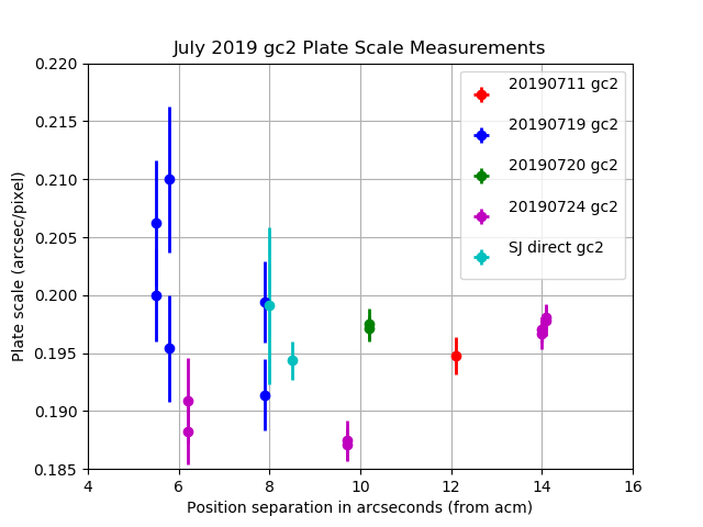
The gc2 plate scales from 4 nights of offset tests. I have also
added direct WCS gc2 measurements made by SJ in early July2019.
Note that the offset data of 20190719 were taken incorrectly (no
allowance for guiding stabilization). I include them for comparison, but
this night was rejected from the mean plate scale values reported here.
|
Overview of the offset method
In this procedure we use sets of simultaneous images obtained with three HET
cameras: the HET acquisition camera (acm) and the two guide probe cameras (gc1,gc2).
Between each set of images, the telescope was offset such that the probe guide stars
remained in their respective fields of view. With well selected target fields, the acm images can
have multiple high S/N star images. The positions of these stars are computed using intensity weighted
centroids. With multiple stars on the acm images we compute high weight offsets (in pixels)
between position sets. We can then derive mean errors for each mean offset measurement. Because
the acm has a well-determined plate scale (ps_acm = 0.2709 ± 0.0001 arcsec/pixel)
from hundreds of WCS derivations, we can convert the measured offsets in pixels to offsets
in units of arcseconds. Similarly, mean centroid measurements are made for the images gathered
with the gc1,gc2 cameras. Offsetting and guiding are all done with the acm, and a sufficient
period is allowed between offsets so that guiding stabilizes. Hence, with each pair of gc image
sets gathered on the sky we can compute an offset in gc image pixels. The acm offset for this
same position pair provides the corresponding offset size in arcseconds. Note that
this method does not depend on the ability of the telescope control system (tcs) to perform
a commanded move. Rather, we simply use the acm images to precisely measure each move after
it is completed and guiding has stabilized. Hence, a plate scale
in units of arcseconds/pixel can be derived for each guide camera (gc1,gc2). We increase the
precision of these measurements by using:
- more stars measured on the acm images
- averaging more images per sky position
Results from this method are given in the previous
section above. More descriptive details follow in the remainder of this report.
Observing Notes
Here I show a few examples of notes made during observing that document
how the test data were gathered. We took sets of acm,gc1,gc2 images with
guiding done on acm. We moved the acm fiducial to perform the telescope
offsets. It should be noted that in the last data set (20190724) we used
7 offsets, with the last two done with no "pid loop". No measurable
difference between the pid and non-pid cases was found. Below we show
the command used for a couple offsets, and the UT times recorded for when
the stabilized image sets were gathered. Detailed observing notes for each
night of offset data are available in other web documents.
Original notes made by SCO:
==================================================================================

20190724
RA: SCO   TO: NM
===========================================================
ENG    gc offset test to derive plate scale

Moon is about 20deg above horizon, and 60% illum

target_setup 54 E -cat gp -ifu 000
This field: 54    GALl110bm5  23:18:39.51  +55:31:29.69     2000  34.3  15.00 06:51 02:11 07:49 01:55

To make acm offsets:
   syscmd -T 'ACQ_offset_fiducial ( dx_asec=5,dy_asec=0,compensate="false")'

Go to target at 06:55 UT
Note DIMM seeing is jumping to 2" just as we get going on this test!

Position START
Starting set of 10 at 07:02:22 UT    (stars centered in gc1,gc2)
Stop taking images at at 07:04:32

Position A
At 7:05
   syscmd -T 'ACQ_offset_fiducial ( dx_asec=5,dy_asec=0,compensate="false")'
*** star moves straight down on gc2
wait for focus and guider stability
Start taking images at   07:08:06 UT
stop 07:10:21

The galpoint field (gp) I used for this is at:   23:18:39.51  +55:31:29.69
high number of stars in the field.
Recall that "galpoint" fields are low galactic latitude fields that
are listed in the htopx "gp" catalog. They are fields we use when we want a
large number of stars in the image field. Fianlly, note that the tcs
trajectory_offset command is made with compensate="false". This means no moves
of the gc probes are performed to keep the guide stars in the same position on
the gc field. The success of this measurement method depends heavily
on the fact that no compensating (or other) motion of the gc probes occurs during
this offsetting of the telescope.
A quick survey of the acm images for the night
You can read about how I reviewed the images in each position/time interval
in a discussion of processing acm images.
In this step I review each set of acm images and delete images that show large
position departures. I then use the final image listing to establish a new
time interval for each position. Since the 20190724 data were by far the best,
I refer to those data in the software examples below, but the same methods were
used in the reducing the other three nights of data. The basic recipe is as follows
I perform this in:  /home/sco/GC_Plate_Scales/20190724

% cat BaseDir
/media/sco/DataDisk1/sco/AD/HET_work/acm_nights
% cat Date
20190724
% cat Time.Sets
  START         07:02:22.0   07:04:32.0
  A             07:08:06.0   07:10:21.0
  B             07:14:24.0   07:16:53.0
  C             07:20:30.0   07:22:47.0
  D             07:30:15.0   07:32:29.0
  E             07:37:00.0   07:39:20.0
  F             07:41:00.0   07:43:33.0
  G             07:45:55.0   07:48:30.0

% pas_time_window_sets acm Time.Sets N
I reject (mark) images with large motions indicated and then rename the list of
unmarked images to an appropriate name. I create a subdirectory with this image file
and record the final range of UT times. These final UT time intervals will be used
to gather the corresponding gc1 and gc2 image sets.
Basically, I build one input file (along with the usual BaseDir and Date files) that
specifies each position name and time interval. For each set the names of images are
collected and run through bigds9, allowing
the user to reject bad images. Note that pas_time_window_sets is not specific to
acm images. Any type of PAS image can be treated. We use it to collect the
gc1 and gc2 images for each position set. The code will form a subdirectory
for each set where the cleaned image lists are stored. Finally, in each set
subdirectory the images are stacked to give a single mean image.
A master set of acm targets.
Typically I will build a mosaic of the stacked fields and use the first image to
set up a set of acm stars that I will measure in each image set. For the subsequent sets
I use the ds9_region_xyshift.sh script
to apply XY shifts that will transform the XY coordinates of the original targets to
the coordinate system of each position set.
% pwd
/home/sco/GC_Plate_Scales/20190724_red2/figs_acm
% ls -1 ../*acm/*.fits >list.acm
   **** I might edit list.acm *****
% bigds9 list.acm 1 10
***
  I blink the images to locate stars that do not leave the field
  or get too close to the image edge to allow centroid calculation.

I save a set of regions for a good image, in this example I save: Eacm.reg
I note the FIRST object I marked in this chart. This is the object I will
identify in all subsequent images for which I'll to build a shifted region file.

Then I create shifted versions of Eacm.reg for each image:
 % ds9_region_xyshift.sh ./Eacm.reg ../STARTacm/STARTacm.fits N
 % ds9_region_xyshift.sh ./Eacm.reg ../Aacm/Aacm.fits N
 etc....

At the end of this process I have the region files for each image.

Now I can rerun bigds9 and then manually load each region file in the
appropriate frame.  I usually copy each region file to its appropriate
subdirectory (with a script).
% bigds9 list.acm 1 10
The two figures below illustrate this mosaic process with bigds9.
 |
|
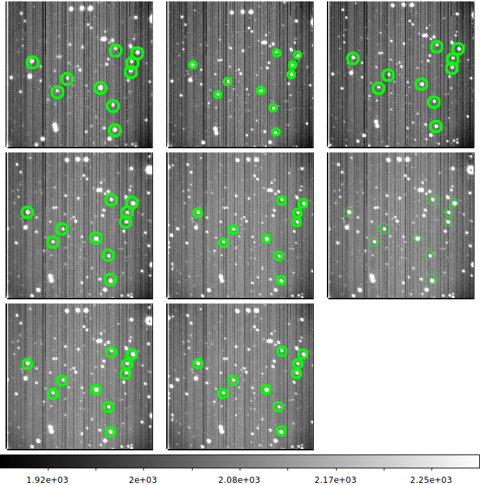
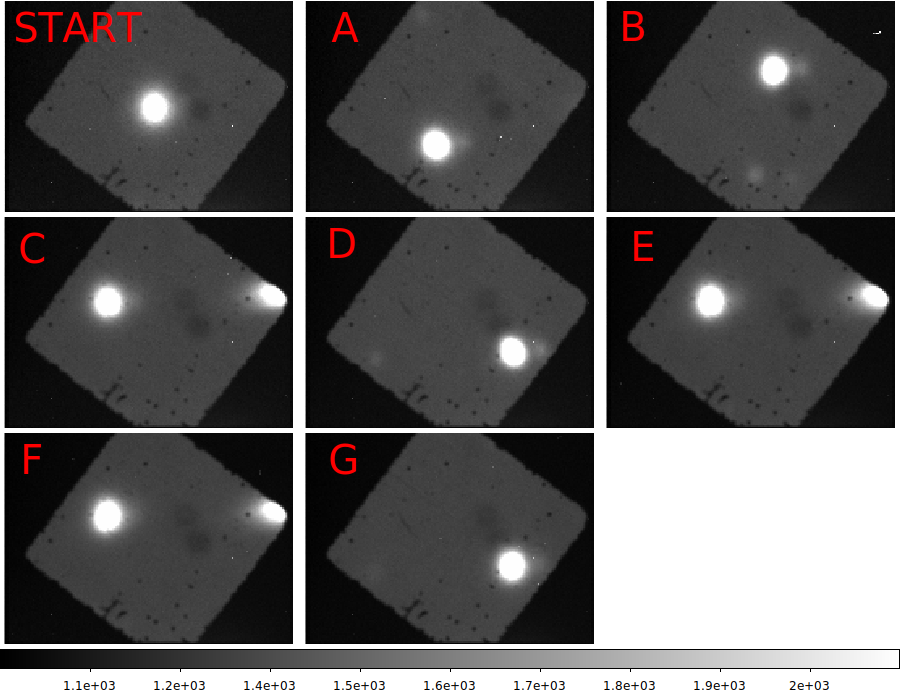
The 8 position fields used in the 20190724 GC offset test. Here I use
the full-field view of each mean image to show that no measurement star is
close to the image edge or leaves the field of view. The top-left image is the
START field, followed in raster fashion by the images for A, B, C, D, E, F, G.
|
 |
|
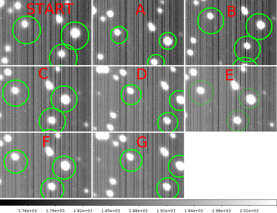
The 8 position fields used in the 20190724 GC offset test. Here I zoom in
on a small portion of the field to show more easily how the image positions
shift. The large red letter indicates the sky position set. Here we can see how
each image position set moves relative to the START position. The largest offsets
on the sky, and hence the best for measuring the GC plate scale values are: A-B,
C-D, and F-G. The F-G sets were made with the pid loop off.
|
Measuring the acm image sets.
The position subdirectories gathered above now contain a list of images
(list.0), a mean stacked image of the field, and an appropriately shifted
region file. In the case of this reduction, each field will have the same
10 stars measured in each image of each position set. For each subdirectory
I would run a command sequence like that below:
% pwd
/home/sco/GC_Plate_Scales/20190724_red2/STARTacm
% ls
list.0	S/  STARTacm.fits  STARTacm.reg
% ds9_imstats_fitslist list.0 FixedRegions N
% ls
list.0	local_red/  S/	STARTacm.fits  STARTacm.reg  XYcenStars.reg  XYmean.parlab  XYmean.reg	XYmean.table
The XYmean.table files are what contain the mean positions and errors of each
of the ten stars we measure in each image. Note that both my own intensity
weighted centroids for each star, as well as the PAS header centroids are stored in these
table files. Unfortunately, with such large position shifts, the PAS stars selected for inclusion
in the header can change from field to field. Hence, the PAS data will occasionally not be useful
in computing mean image position shifts. The two figures below illustrate the measurements made
by ds9_imstats_fitslist.
 |
|
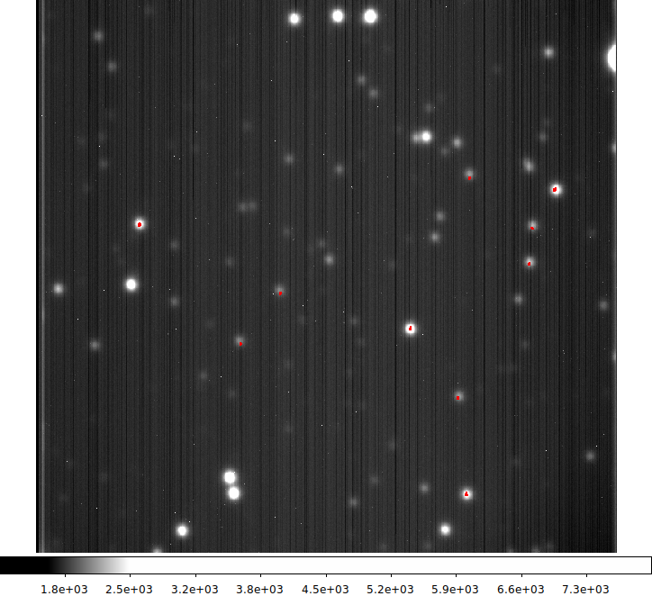
Here is the full-field view of our stacked START field. The ten stars that have
been measured in each of the eight images for this field have small red circles
plotted above to indicate the XY values of the intensity-weighted position centroids.
Note that for the single star measured in the PAS image headers, I have made extensive
comparisons with the intensity weight centroids measured with ds9_imstats_fitslist,
and found no systematic difference.
|
 |
|
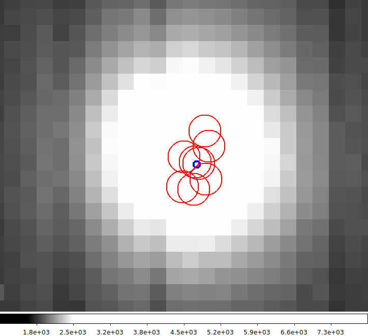
This is a zoomed-in view of one star in the previous figure. We see the
8 red dots indicating the centroid positions measured on each of the 8 input images.
The thick blue circle indicates the mean of these positions. The median position
and the error of the mean are also stored in the XYmean table files. With these data
we can determine high-weight estimates for the sky offsets (in pixel units) between
two position sets. Given the high S/N of the stars used in ech image, the scatter of the
red points is not due to measurement error, but rather represents motion on the sky of
the PSF averaged over the time of observation. In this cases we gathered 8 images at 6
seconds per exposure, and hence, the motion represents that for a total period of 48 seconds.
At the time these data were taken the HET DIMM was measuring just under 1.75 to 2.0
arcseconds. For this image the X,Y errors combined in quadrature indicate a mean error
of ±0.22 pixels or ±0.06 arcseconds. Hence, assuming comparable errors in
another image set, our offset errors should be about ±0.08
arcseconds.
|
To measure position offsets
With mean positions and errors computed for each set of positions, we can now
use pairs of positions to compute offsets on the sky. The gc offsets will be
in units of pixels, and the acm offsets will also be in pixels, but will be
converted to units of arcseconds in a later section when plate scale estimates
are derived.
To compute the possible sets of offsets:
    cd /home/sco/GC_Plate_Scales/20190724_red2
    table_XY_offsets.sh ./Aacm/XYmean ./Bacm/XYmean xmean ymean xme yme N
    pas_XY_offsets.sh ./Aacm/list.0 ./Bacm/list.0 1.0  N

An easy script run:     ./S/ORUN Aacm Bacm
                        ./S/ORUN STARTacm Eacm
                        ./S/ORUN Cacm Dacm
                        ./S/ORUN Gacm Facm

Here I collect the acm position set offsets

           SCO centroid                                     PAS centroids                      Position Pair
     mean        median          m.e.  Nstar        mean         median        m.e.   Nims
     ---------------------------------------       ---------------------------------------
     35.719       35.959        0.293    10         37.156       37.256        0.519     8     A-B
     22.979       22.745        0.352    10         21.989       22.293        0.803     8     START-E
     52.101       52.203        0.112    10         52.159       52.421        0.454     8     C-D
     51.679       51.715        0.068    10         51.658       51.751        0.494    10     G-F
Measuring the gc1 image sets.
Because the gc images normally contain only a single bright star, the
measurement of these images is less complicated than the acm sets.
 *** Gather the position set subdirectories ********
There are N=3423 gc1 images
% pwd
/home/sco/GC_Plate_Scales/20190724_red2
% ls
BaseDir  Date  S/  Time.Sets
% cat BaseDir
/media/sco/DataDisk1/sco/AD/HET_work/acm_nights
% cat Date
20190724
% cat Time.Sets_refined
  START         07:02:39.7  07:04:18.3
  A             07:08:31.0  07:10:09.6
  B             07:14:50.5  07:16:43.1
  C             07:20:56.0  07:22:34.7
  D             07:30:32.0  07:32:24.7
  E             07:37:19.4  07:39:12.1
  F             07:41:18.4  07:43:25.0
  G             07:46:13.5  07:48:20.3
% pas_time_window_sets gc1 Time.Sets_refined N

% pwd
/home/sco/GC_Plate_Scales/20190724_red2/figs_gc1
% ls -1 ../*gc1/*.fits >list.gc1
   **** I might edit list.acm *****
% bigds9 list.gc1 1 10

*** In each subdirectory for gc1
% ds9_imstats_fitslist list.0 FixedRegions N

To compute the possible sets of offsets:
    cd /home/sco/GC_Plate_Scales/20190724_red2
    table_XY_offsets.sh ./Agc1/XYmean ./Bgc1/XYmean xmean ymean xme yme N
    pas_XY_offsets.sh ./Agc1/list.0 ./Bgc1/list.0 1.0  N

An easy script run:     ./S/ORUN Agc1 Bgc1
                        ./S/ORUN STARTgc1 Egc1
                        ./S/ORUN Cgc1 Dgc1
                        ./S/ORUN Ggc1 Fgc1

Here I collect the gc1 position set offsets

           SCO centroid                                     PAS centroids                      Position Pair
     mean        median          m.e.  Nstar        mean         median        m.e.   Nims
     ---------------------------------------       ---------------------------------------
     51.748       51.748        0.403     1          51.296       51.381        0.532    20    A-B
     32.049       32.049        0.501     1          32.001       31.901        0.660    20    START-E
     71.346       71.346        0.421     1          71.235       71.287        0.466    19    C-D
     71.227       71.227        0.417     1          70.705       70.868        0.521    24    G-F
 |
|
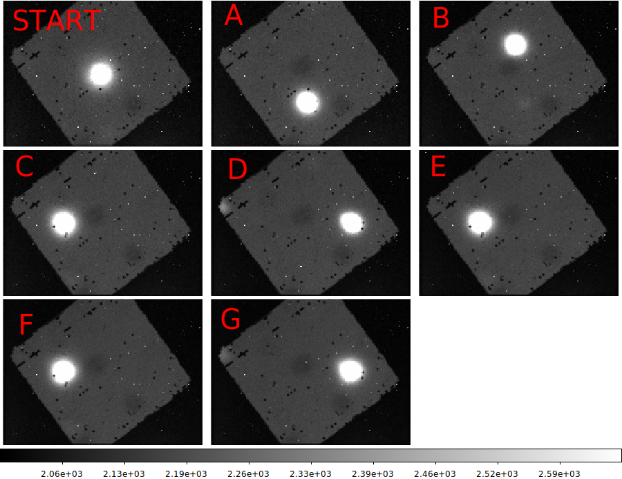
The mean (stacked) gc1 images. The position set is indicated by the large red letter.
|
Measuring the gc2 image sets.
Here I present the same procedure for gc2.
*** Gather the position set subdirectories
******** There are N=3821 gc2 images
% pwd
/home/sco/GC_Plate_Scales/20190724_red2
% ls
BaseDir  Date  S/  Time.Sets
% cat BaseDir
/media/sco/DataDisk1/sco/AD/HET_work/acm_nights
% cat Date
20190724
% cat Time.Sets_refined
  START         07:02:39.7  07:04:18.3
  A             07:08:31.0  07:10:09.6
  B             07:14:50.5  07:16:43.1
  C             07:20:56.0  07:22:34.7
  D             07:30:32.0  07:32:24.7
  E             07:37:19.4  07:39:12.1
  F             07:41:18.4  07:43:25.0
  G             07:46:13.5  07:48:20.3
% pas_time_window_sets gc2 Time.Sets_refined N

% pwd
/home/sco/GC_Plate_Scales/20190724_red2/figs_gc2
% ls -1 ../*gc2/*.fits >list.gc2
   **** I might edit list.acm *****
% bigds9 list.gc2 1 10

*** In each subdirectory for gc1
% ds9_imstats_fitslist list.0 FixedRegions N

To compute the possible sets of offsets:
    cd /home/sco/GC_Plate_Scales/20190724_red2
    table_XY_offsets.sh ./Agc1/XYmean ./Bgc1/XYmean xmean ymean xme yme N
    pas_XY_offsets.sh ./Agc2/list.0 ./Bgc2/list.0 1.0  N

An easy script run:     ./S/ORUN Agc2 Bgc2
                        ./S/ORUN STARTgc2 Egc2
                        ./S/ORUN Cgc2 Dgc2
                        ./S/ORUN Ggc2 Fgc2

Here I collect the gc2 position set offsets

           SCO centroid                                     PAS centroids                      Position Pair
     mean        median          m.e.  Nstar        mean         median        m.e.   Nims
     ---------------------------------------       ---------------------------------------
     51.715       51.715        0.383     1        51.617       51.526        0.477    20      A-B
     33.071       33.071        0.498     1        32.604       32.629        0.627    20      START-E
     71.238       71.238        0.385     1        71.347       71.620        0.457    20      C-D
     71.079       71.079        0.398     1        71.171       71.451        0.520    24      G-F
 |
|
The mean (stacked) gc2 images. The position set is indicated by the large red letter.
|
Plate scales are measured.
The plate scale values derived from offsets are computed using the offsets in pixels
between each pair of gc1/gc2 image sets, and offsets in arcseconds using each pair of
acm image positions.
 % pwd
Working location: /home/sco/GC_Plate_Scales/20190724_red2/PS_estimates

Build a file named 20190724.dat:
% cat 20190724.dat
A-B
     35.719       35.959        0.293    10         37.156       37.256        0.519     8     A-B
     51.748       51.748        0.403     1          51.296       51.381        0.532    20    A-B
     51.715       51.715        0.383     1        51.617       51.526        0.477    20      A-B
START-E
     22.979       22.745        0.352    10         21.989       22.293        0.803     8     START-E
     32.049       32.049        0.501     1          32.001       31.901        0.660    20    START-E
     33.071       33.071        0.498     1        32.604       32.629        0.627    20      START-E
C-D
     52.101       52.203        0.112    10         52.159       52.421        0.454     8    C-D
     71.346       71.346        0.421     1          71.235       71.287        0.466    19    C-D
     71.238       71.238        0.385     1        71.347       71.620        0.457    20      C-D
G-F
     51.679       51.715        0.068    10         51.658       51.751        0.494    10    G-F
     71.227       71.227        0.417     1          70.705       70.868        0.521    24    G-F
     71.079       71.079        0.398     1        71.171       71.451        0.520    24      G-F

Next we compute the plate scale values
% gcps.sh 20190724.dat N

To make a plot of the estimates (for example):
 % Generic_Points N
 % xyplotter_auto gc1_plate_scales q q 1 N
   (edit Axws.1 List.1)
 % xyplotter List.1 Axes.1 N

I add the plot data to my older 3 set analysis in: /home/sco/GC_Plate_Scales/4sets

  xyplotter xyplotter List.1 Axes.1 N
  xyplotter xyplotter List.2 Axes.2 N
Plots of the data prepared in this way are shown near the beginning of this report.
Final weighted mean values.
The plate scale values for the offsets from the previous section were gathered
into single gc1,gc2 files. I also added gc plate scale measurements
from direct WCS solutions made by SJ in early July2019. I have added these direct
results (2 fields on two different nights) to the plots (the "SJ" cyan points)
and have added them as independent measurements in computing the final weighted
mean values and errors. Note that for the offset cases, I refer to these data as
being from "Stable" nights since the proper wait times between images sets were
used to allow guiding to stabilize before the image sets were recorded.
% pwd
/home/sco/GC_Plate_Scales/4sets/Only_Stable_Nights

I derive weighted mean stats for the 4 stable offset nights (20190711,20190720,20190724)
and the SJ wcs solutions from two nights (20190712,20190713)

GC1:
PS values from stable data nights
   Pair    cam   meth    Sep      ps     m.e.    date
# data
    AB      gc1   sco   12.1    0.1973  0.0015   20190711
    AB      gc1   sco   10.2    0.1989  0.0012    20190720
    AB      gc1   pas   10.2    0.1989  0.0013    20190720
    AB      gc1   sco    9.7    0.1870  0.0015    20190724
    AB      gc1   pas    9.7    0.1886  0.0020    20190724
    STE     gc1   sco    6.2    0.1942  0.0030    20190724
    STE     gc1   pas    6.2    0.1945  0.0040    20190724
    CD      gc1   sco   14.1    0.1978  0.0012    20190724
    CD      gc1   pas   14.1    0.1981  0.0013    20190724
    GF      gc1   sco   14.0    0.1966  0.0012    20190724
    GF      gc1   pas   14.0    0.1980  0.0015    20190724
   SJx      gc1   dir    8.0    0.1950  0.0014    20190712
   SJy      gc2   dir    8.5    0.1953  0.0032    20190712
   SJx      gc1   dir    9.0    0.1943  0.0023    20190713
   SJy      gc2   dir    10.0   0.1944  0.0012    20190713


GC2:
Stable night gc2 estimates
   Pair    cam   meth    Sep      ps     m.e.
# data
    AB      gc2   sco   12.1    0.1948  0.0016   20190711
    AB      gc2   sco   10.2    0.1971  0.0011   20190720
    AB      gc2   pas   10.2    0.1975  0.0013   20190720
    AB      gc2   sco    9.7    0.1871  0.0014   20190724
    AB      gc2   pas    9.7    0.1875  0.0017   20190724
    STE     gc2   sco    6.2    0.1882  0.0028   20190724
    STE     gc2   pas    6.2    0.1909  0.0037   20190724
    CD      gc2   sco   14.1    0.1981  0.0011   20190724
    CD      gc2   pas   14.1    0.1978  0.0013   20190724
    GF      gc2   sco   14.0    0.1970  0.0011   20190724
    GF      gc2   pas   14.0    0.1967  0.0014   20190724
   SJx      gc2   dir    8.0    0.1991  0.0067   20190713
   SJy      gc2   dir    8.5    0.1944  0.0017   20190713
In the tables above, "meth" refers to the method used to derive the X,Y centroids
in each image. The "sco" value refer to my own code that measures multiple sets of stars
(if present), and "pas" refers to values taken from the PAS image headers.
Both sets are intensity-weight centroids. The second method was sometimes
incomplete when image measurement (metrology) was not activated during data taking, or
when different gc stars were measured in offset image pairs.
The values with "meth=dir" are the WCS solution values from SJ.
The values of "Sep" indicate the size of the offset in units of arcseconds.
The values of "ps" are the plate scale estimates in units of arcsec/pixel.
The base names of my table files are:   PS_gc1 , PS_gc2

% table_stats.sh PS_gc1 ps pserr N
mean,median,sigma,m.e.,n:
      0.195260       0.195300       0.003490       0.000901     15
Weighted estimates (mean,sigma,m.e):
      0.195992       0.003430       0.000886

% table_stats.sh PS_gc2 ps pserr N
mean,median,sigma,m.e.,n:
      0.194323       0.196700       0.004359       0.001209     13
Weighted estimates (mean,sigma,m.e):
      0.195328       0.003875       0.001075
These mean plate scale values are reported in the results section
near the beginning of this report.
Back to calling page