May 2020 notes: photometry calibration
Last updated: May12,2020
- Calibrating the acm photometry
- Making a table file
- Diagnosing a set of i images
- Plotting by filter and date
- How many times can I do this?
Calibrating the acm photometry
In AprilMay of 2020 I began to develop a new generation of routines
for calibrating acm photomtery primarily for the purpose of measuring
night sky surface brightness in a standard photometric system. The
basic steps are summarized below.
Reduction location:  /home/sco/ACM_work_Oct2019

In a given date subdirectory:
   cat ./local_red/ISET_STACKS/list.* > List.1
   phot2_fitslist List.1 0.05 3

To generate a quick and klugy phot2 table file for the plot below:
   cd /home/sco/ACM_work_Oct2019
   gethead -u -f 20*/local_red/PHOT2/*.fits PSYSNAME ZPSEC ZPERR NUMZP SKYSB SKYSBERR VSKYSB  >phot2.table

I manually generated the phot2.parlab file and then used some munging tools to
divide the table into Tg and Ti tables.
Some initial results are summarized in the figure below.
 |
|
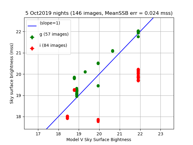
The calibarted sky surface brightness measured from acm images gathered
during 5 nights in Oct2019. These nights were mostly dark and extremely clear.
The g points follow a resonable trend, but the i data points are clearly
suffering some kind of error at the bright end.
|
Return to top of page.
Making a table file
Here is a way to make a table file.
% pwd
/home/sco/ACM_work_Oct2019/phot2_check_3
% ls -1 ../red_20*/local_red/PHOT2/*.fits > list.0
% install_pimag_fitslists list.0 N
% mkdir PHOT2_local
% mv *.fits PHOT2_local
% ls -1 ./PHOT2_local/20*.fits > list.0

# This makes a list of 146 calibrated (PHOT2) images with the PIMAG card installed
# I move this images in a local subdirectory named ./PHOT2_local. This is not so
# efficient, but it has the advantage that the images are held locally and I can
# make plots with this set and not worry about the images in the ../red_* directories
# being changed.

Here is a way to make the parameter lists:
I manually list the FITS header parameters of interest:
% cat Data1.params
PSYSNAME
SKYSB
SKYSBERR
ZPSEC
ZPERR
NUMZP
MILLUM
PHIMOON
VSKYSB
PUPILLUM
RSTRT
PIMAG

I use the make_parlabs routine to build the parlabs file
% make_parlabs Data1
% cat Data1.parlab
PSYSNAME     name of photometric system
SKYSB     sky surface brightness (mags per sq.arcsec)
SKYSBERR     mean error of SKYSB
ZPSEC     ZP for a 1-sec exposure
ZPERR     mean error of ZPSEC
NUMZP     number of ZP calbration sources
MILLUM     ercentage moon illumination
PHIMOON     ngle of separation to moon (deg)
VSKYSB     model V sky surface brightness (mss)
PUPILLUM     Pupil illumination relative to ITF 0
RSTRT     Radius position of tracker at start (mm)
PIMAG     Pupil illuminationn magnitude units

**** NOTE: You could just manually build the file named Data1.parlab,
           but the parameter labels in $critfils are more universal.
% cp Data1.parlab P.list

% ls
list.0	 P.list

% fits2table list.0 P.list Data1 N
% ls
Data1.images  Data1.params  Data1.parlab  Data1.table  list.0  P.list

To just make plots:
% xyplotter_auto Data1 q q 10 N
**** I used this to make the two plots below.
To replot thisng with samll adjustments to List.10 and/or Axes.10
% xyplotter List.10 Axes.10 N

To view the parameter spcae and view selected images with ds9:
% point_selector Data1 VSKYSB SKYSB N
This works, but point_selector uses the same point symbol, so it is impossible to
indentify g and i points. We want to investiagte the weird i data points, so here is
a slightly klugy way to do this using existig tools.
% cat Rules.i
PSYSNAME   text     i     none

I make a new table fril with basename = iData
% cat Rules.i
PSYSNAME   text     i     none

% table_mask_builder Data1 Rules.i iData N
  89     final_number

% ls
Data1.images  Data1.parlab  iData.images  iData.parlab	Last.BoxLims  P.list   S/	    Viewed.Images  xyf.old
Data1.params  Data1.table   iData.params  iData.table	list.0	      Rules.i  subdir.path  xyf.in

**** The table we want to use now is:   iData
% point_selector iData VSKYSB SKYSB N

I marked a set of i images clumped at a strange position in the SKYSB vs. VskySB space.
Impornat Conclusion:  Thye are all of the same field!

I marked them and said "Y" to recording them, so noew I see:
% cat Viewed.Images
../red_20191020/local_red/PHOT2/20191020T113202.9_acm_sci.fits
../red_20191020/local_red/PHOT2/20191020T113153.1_acm_sci.fits
../red_20191020/local_red/PHOT2/20191020T113125.8_acm_sci.fits
../red_20191020/local_red/PHOT2/20191020T113134.9_acm_sci.fits
../red_20191020/local_red/PHOT2/20191020T113144.1_acm_sci.fits

Another useful thing:
* Mark points with the "b" (box) option, then make two
  tables of the marked and unmarked files. In addition, I
  get the images lists for each of these sets.

% ls
iData.images  iData.params  iData.parlab  iData.table  xyf.in

% split_table_by_selector iData N

HINT: Try moving the ds9 window to another monitor.

% ls
data_strip.out	iData.params  iData.table  Marked.images  Marked.table	    NotMarked.parlab  XYF
iData.images	iData.parlab  lines.NO	   Marked.parlab  NotMarked.images  NotMarked.table   xyf.in

*** I marked a clump of 5 points, and here they are:
% cat Marked.images
../red_20191020/local_red/PHOT2/20191020T113125.8_acm_sci.fits
../red_20191020/local_red/PHOT2/20191020T113134.9_acm_sci.fits
../red_20191020/local_red/PHOT2/20191020T113144.1_acm_sci.fits
../red_20191020/local_red/PHOT2/20191020T113153.1_acm_sci.fits
../red_20191020/local_red/PHOT2/20191020T113202.9_acm_sci.fits
Hence, the question is: what is wrong with this image set from 20191020? Actually, further
inspection shows me that the 3 clumps of points in the bright sky i data are of 3 distinct
sky positions. So, I am seeing a lot of variation of i sky SB measurements when the moon
is up.
 |
|
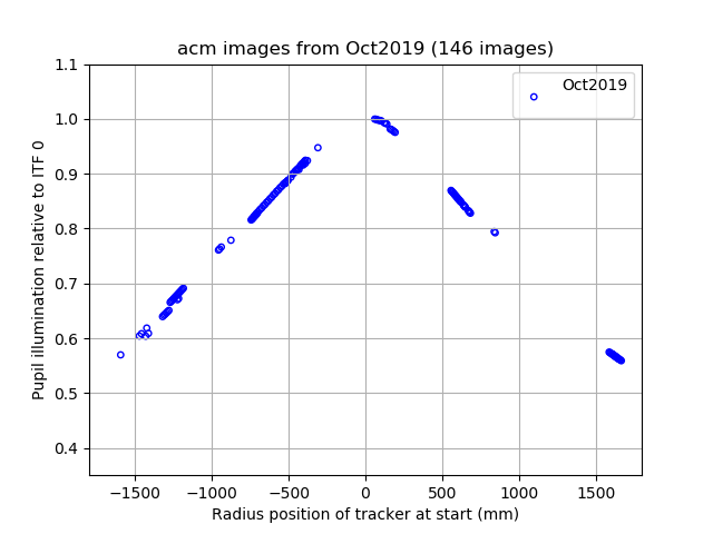
The pupil illumination percentage (PUPILLUM) as a fuction of tracker offset
from center (RSTRT) for the 146 images reduced from 5 nights in Oct2019.
|
 |
|
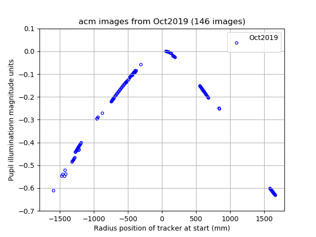
The pupil illumination percentage in units of magnitudes (PIMAG) as a fuction of
tracker offset from center (RSTRT) for the 146 images reduced from 5 nights in
Oct2019.
|
 |
|
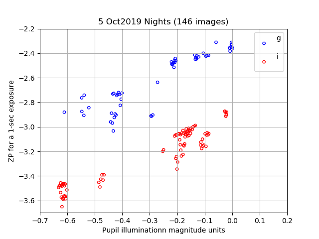
The g,i zero point values (ZPSEC) as a function of pupil illumination percentage in
units of magnitudes (PIMAG). These points are from 5 nights in Oct2019. The weather
was judged extremely clear.
|
Return to top of page.
Diagnosing a set of i images
The plot below shows about 80 measurements of i sky surface brightness
values as a function of predicted V sky surface brightness. The Vsky model may
not be very realistic, but it does let us see which points were obtained
when the moon was up. The 3 clumps of points that are brighter than
Vsky=20 are from three different sky positions. The points marked in blue
are the most discrepant (i.e. much to faint for a bright moon sky) and we'll
concentrate in this sections on diagnosing this set of image photometry.
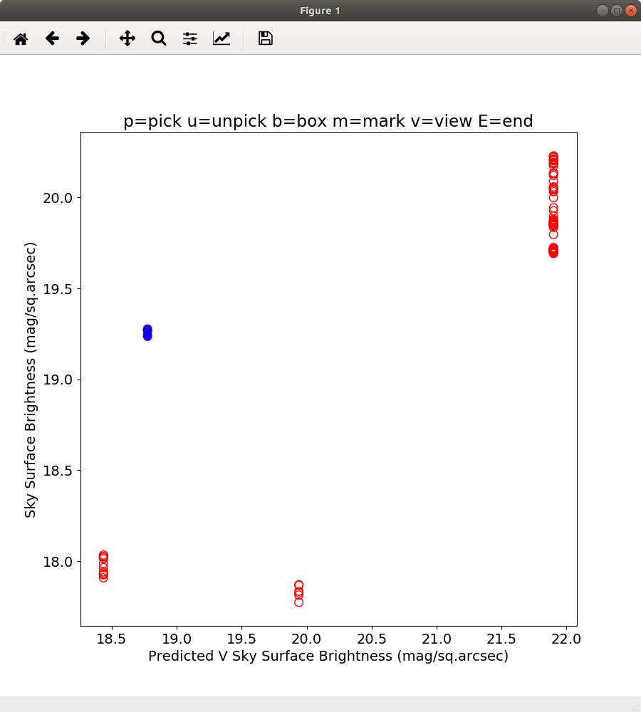 |
This plot of observed i sky surface brightness vs. model V sky surface brightness
was made with the point_selector call shown below. I identified 5 points and isolated the
image names associated with these points using split_table_by_selector. The list of 5 images is
show below:
% point_selector iData VSKYSB SKYSB N
% split_table_by_selector iData N
% mv Marked.images badi_1.list
% cat badi_1.list
../red_20191020/local_red/PHOT2/20191020T113125.8_acm_sci.fits
../red_20191020/local_red/PHOT2/20191020T113134.9_acm_sci.fits
../red_20191020/local_red/PHOT2/20191020T113144.1_acm_sci.fits
../red_20191020/local_red/PHOT2/20191020T113153.1_acm_sci.fits
../red_20191020/local_red/PHOT2/20191020T113202.9_acm_sci.fits
The question now is: why are these image from one pointing on the night of
20191020 giving sky surface brightness values that appear to be overly dark?
|
It would seem the first step is to just use the existing code to rederive the
ZP and sky brightness estimates using phot2_fitslist, but running in an interactive
mode (using the "-i" flag) so that we can view each set of points used to derive
the mean zeropoint of each image.
% cat list.0
../red_20191020/local_red/PHOT2/20191020T113144.1_acm_sci.fits
% phot2_fitslist list.0 0.05 3 -i

Old:   i sky surface brightness = 19.24  -+0.04 mss
New:   i sky surface brightness = 19.24  -+0.03 mss

Here are some useful header cards for the re-reduced image:
ZPSEC   =              -2.9135 / ZP for a 1-sec exposure
ZPERR   =               0.0413 / mean error of ZPSEC
NUMZP   =                   15 / number of calbrating sources

SKYMEAN =            506.26157 / mean sky in adu (skymap2)
SKYME   =              0.04432 / error of mean sky in adu

SKYSB   =              19.2360 / sky surface brightness (mags per sq.arcsec)
SKYSBERR=               0.0410 / mean error of SKYSB

MILLUM  =             66.4000 / percentage moon illumination
PHIMOON =             36.9672 / angle of separation to moon (deg)
VSKYSB  =             18.7750 / predicted V sky surface brightness
Using a radius=4" aperture, I re-mesure the photometry and interactively fit the
ZP, and I find very little difference with the old (automated) derivation. Moreover,
a total of 15 stars was used in the ZP calculation. Notice from the FITS header cards
that the moon was 66% illuminated and we were only 37 degrees from the moon when the
image was taken. It is hard to believe the i-band sky was really this faint when the
image was taken.
Next, I use ds9_imstats to inspect the image
and manually measure some sky boexs and stars:
% pwd
/home/sco/ACM_work_Oct2019/red_20191020
% ds9_imstats ./local_red/PHOT2/20191020T113144.1_acm_sci.fits Y

# Contents of:  midodata.2
Col01 = X pixels (aperture X center)
Col02 = Y pixels (aperture Y center)
Col03 = X center, pixels (intensity weighted centroid)
Col04 = Y center, pixels (intensity weighted centroid)
Col05 = magnitude (assuming zp=30)
Col06 = Average value per pixel in aperture
Col07 = Average value per pixel in annulus
Col08 = number of pixels in aperture
Col09 = Peak pixel value (no bkg-sub, image ADU)
Col10 = marker code (1=circle,2=box,3=ellipse)
                                                 Aperture   Annulus                Peak
   456.88    501.84    447.31    496.18  14.039  1178.514   513.564     3645.0   55055.23   2     green
   505.20    391.12    501.03    389.33  14.651   968.881   515.498     3042.0   29020.07   2     green
   291.30    242.28    275.51    232.52  12.313  1797.013   525.760     9345.0   64185.41   2     green

   388.97    419.47    343.00    389.00 -99.000   516.140   631.069     9191.0     633.21   2     red
   542.15    263.11    539.35    260.32  20.063   512.649   511.692     9855.0     655.32   2     red

% cat a.1
516.140
631.069
512.649
511.692

% calstats.py a.1 -v
Simple stats for numbers in: a.1
Mean                     = 542.88750
Median                   = 514.39450
Standard deviation       = 50.93852
Minimum                  = 511.69200
Maximum                  = 631.06900
Number of values         = 4
Mean error of then mean  = 29.40937
The first 3 red boxes contained stars, and we see that in two cases the pek flux values are
near saturation (55K and 64K) so this means the ZP could be poor. The median of the two (red) sky
boxes (using aperture and annuli) would be: MeanSky = 514.39 -+ 29.4.
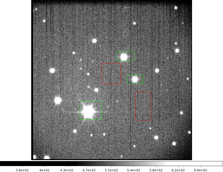 |
The acm i image measures in the above exercise.
% pwd
/home/sco/ACM_work_Oct2019/red_20191020
% ds9_imstats ./local_red/PHOT2/20191020T113144.1_acm_sci.fits Y

# Contents of:  midodata.2
Col01 = X pixels (aperture X center)
Col02 = Y pixels (aperture Y center)
Col03 = X center, pixels (intensity weighted centroid)
Col04 = Y center, pixels (intensity weighted centroid)
Col05 = magnitude (assuming zp=30)
Col06 = Average value per pixel in aperture
Col07 = Average value per pixel in annulus
Col08 = number of pixels in aperture
Col09 = Peak pixel value (no bkg-sub, image ADU)
Col10 = marker code (1=circle,2=box,3=ellipse)
                                                 Aperture   Annulus                Peak
   456.88    501.84    447.31    496.18  14.039  1178.514   513.564     3645.0   55055.23   2     green
   505.20    391.12    501.03    389.33  14.651   968.881   515.498     3042.0   29020.07   2     green
   291.30    242.28    275.51    232.52  12.313  1797.013   525.760     9345.0   64185.41   2     green

   388.97    419.47    343.00    389.00 -99.000   516.140   631.069     9191.0     633.21   2     red
   542.15    263.11    539.35    260.32  20.063   512.649   511.692     9855.0     655.32   2     red
We could have problems with a bad ZP value caused by image saturation in the bright stars.
How do the ZP values for this image (images!) compare to the other images?
|
Return to top of page.
Plotting by filter and date
Here I use table files to build a big table and plot parts of it.
# I did this work in:   /home/sco/ACM_work_Oct2019/phot2_check_3/T0

fits2table list.0 P.list TAB0 N
table_PAS_times.sh list.0 TAB1 N
table_merge TAB0 TAB1 ACM N

To get a table of a specific filter on a given date:
% cat rules
UTdate    text   20191018   none
PSYSNAME  text   i          none
% table_mask_builder ACM rules 20191018i N
  35     final_number

% xyplotter_auto 20191018i PIMAG ZPSEC 200 N
% xyplotter_auto 20191018g PIMAG ZPSEC 200 N

To do the table_mask_builder part:
% cat setget

#!/bin/bash
# Check command line arguments
if [ -z "$1" ]
then
 printf "Usage: setget 20191020 i \n"
 printf "arg1 - date string   \n"
 printf "arg2 - filter (g,r,i,B,V,R) \n"
 exit
fi
if [ -z "$2" ]
then
 printf "Usage: setget 20191020 i \n"
 printf "arg2 - filter (g,r,i,B,V,R) \n"
 exit
fi

date="$1"
filter="$2"

printf  "UTdate  text  $date   none \m" > rules
printf  "PSYSNAME   text  $filter   none \n" >> rules

fo="$date$filter"
table_mask_builder ACM rules $fo N


To run the script:
% setget 20191020 i
  5     final_number
% setget 20191020 g
  12     final_number

Then I add to the List.200 file to add the sets.
% cat List.200
20191018i.table 13 5 0 0   pointopen   r o 45    20191018i
20191018g.table 13 5 0 0   pointopen   b o 45    20191018g
20191020i.table 13 5 0 0   pointopen   r s 45    20191020i
20191020g.table 13 5 0 0   pointopen   b s 45    20191020g
20191022i.table 13 5 0 0   pointopen   r ^ 45    20191022i
20191022g.table 13 5 0 0   pointopen   b ^ 45    20191022g
20191026i.table 13 5 0 0   pointopen   r D 45    20191026i
20191026g.table 13 5 0 0   pointopen   b D 45    20191026g
20191027i.table 13 5 0 0   pointopen   r H 45    20191027i

% cat Axes.200
146 acm images (5 clear nights in Oct2019)
  -0.8 +0.05            Pupil illumination in magnitude units
  -5.34450 -0.03170     ZP for a 1-sec exposure

To make the plot:      xyplotter List.200 Axes.200 N
The resultant plot is shown below.
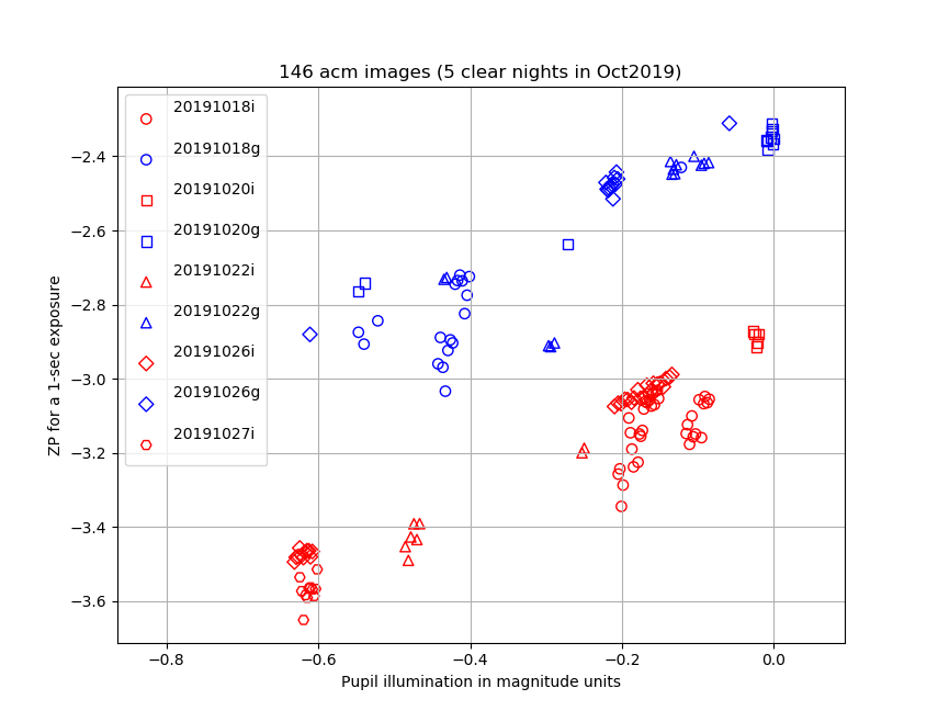 |
The g,i zeropoint values (ZPSEC) as a function of pupil illumination in units of
magnitudes (PIMAG). The night dates are denoted by point symbol and the
filters are denoted by color (i images in RED, g images in BLUE). Some discrepant
points are present, but the ZP values change by a little over a half magnitude from the
tracker center to the outer regions. I am currently checking whether some of the more
discrepant points could be due to clouds (May12,2020). Using these zeropoints, global
sky estimates for each image, and using only (g,i) images taken when the moon was
down we obtain these sky surface brightness statistics:
   filter    Mean     Median    m.e.   Number
     g       21.97     22.01    0.02    16
     i       19.92     19.86    0.02    66
|
Return to top of page.
How many times can I do this?
I built a new fitsfind routine (fitsfind_markII)
that I can use to build a file of full path imag names. I also wanted to add some new
parametrs to me table files (EXPTIME and STRUCTAZ), so I spiffed up the files in
$critfils/paramlabels/ and remade my P.list file with make_parlabs.
I do this in:  /home/sco/ACM_work_Oct2019/phot2_check_4

First I start with a (fullpath) list of images that I created yesterday that
have the PIMAG cards installed in the FITS headers:
% fitsfind_markII ../phot2_check_3/PHOT2_local/ -fp -p 2019
 146    (Number of FITS file found, see fitsfind.out)
% mv fitsfind.out list.0
% head -5 list.0
/home/sco/ACM_work_Oct2019/phot2_check_3/PHOT2_local/20191018T024537.2_acm_sci.fits
/home/sco/ACM_work_Oct2019/phot2_check_3/PHOT2_local/20191018T061517.4_acm_sci.fits
/home/sco/ACM_work_Oct2019/phot2_check_3/PHOT2_local/20191018T061348.5_acm_sci.fits
/home/sco/ACM_work_Oct2019/phot2_check_3/PHOT2_local/20191020T065236.9_acm_sci.fits
/home/sco/ACM_work_Oct2019/phot2_check_3/PHOT2_local/20191022T032114.9_acm_sci.fits

% cat P.params
PSYSNAME
SKYSB
SKYSBERR
ZPSEC
ZPERR
NUMZP
MILLUM
PHIMOON
VSKYSB
PUPILLUM
RSTRT
PIMAG
EXPTIME
STRUCTAZ

% make_parlabs P
% cat P.parlab
PSYSNAME     name of photometric system
SKYSB     sky surface brightness (mags per sq.arcsec)
SKYSBERR     mean error of SKYSB
ZPSEC     ZP for a 1-sec exposure
ZPERR     mean error of ZPSEC
NUMZP     number of ZP calbration sources
MILLUM     ercentage moon illumination
PHIMOON     ngle of separation to moon (deg)
VSKYSB     model V sky surface brightness (mss)
PUPILLUM     Pupil illumination relative to ITF 0
RSTRT     Radius position of tracker at start (mm)
PIMAG     Pupil illuminationn in magnitude units
EXPTIME     integration time (seconds)
STRUCTAZ     Azimuth of HET structure (degrees)
% cp P.parlab P.list

% fits2table list.0 P.list TAB0 N
% table_PAS_times.sh list.0 TAB1 N
% table_merge TAB0 TAB1 ACM N
% table_checker ACM N
% ls ACM*
ACM.images  ACM.params	ACM.parlab  ACM.table

Make a plot from this table and view images using the "v" key.
% point_selector ACM PIMAG ZPSEC N

Just make a plot and pick my parameters interactively:
% Generic_Points N
% xyplotter_auto ACM q q 20 N

% pwd
/home/sco/ACM_work_Oct2019/phot2_check_4/Look1
% ls
ACM.images  ACM.params	ACM.parlab  ACM.table

I can split the tables up:
% acm_setget 20191018 g
  18     final_number
20191018g.images  20191018g.params  20191018g.parlab  20191018g.table

If we look at the local directory now:
% ls
20191018g.images  20191018g.params  20191018g.parlab  20191018g.table  ACM.images  ACM.params  ACM.parlab  ACM.table  rules

I can inspect the g image from 20191018:
% point_selector 20191018g PIMAG ZPSEC N
This was the process I used on May13,2020 and in the course of this I found a set
of g image from 20191018 taken at one sky position. A few of the points from
the set in a ZPSEC vs. PIMAG plot showed a wide scatter. I tracked this to the
fatc that some of the image had very poor focus. I used a modicied version
of the ds9_profiles code to compute
profiles that demonstrate this in the figures below.
 |
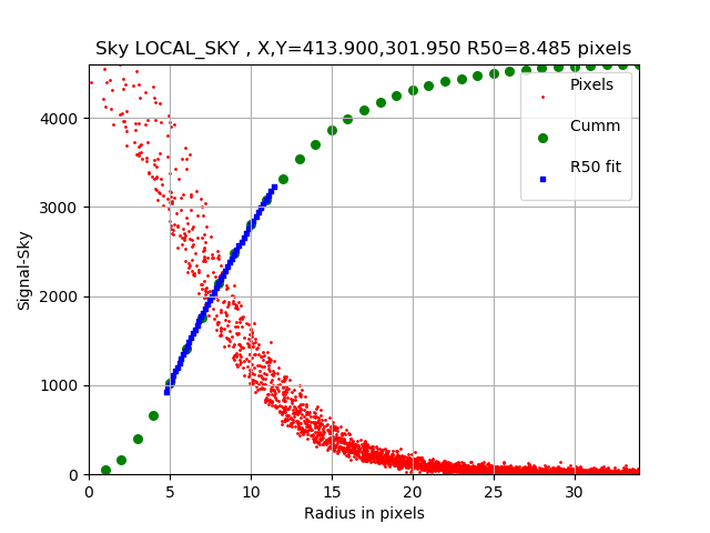 |
Image in the g filter from 20191018. The top profile is from an image that was in good focu and the
bottom profile is from a poorly focused image.
Good focus (T0_good_focus):
ds9_profiles_x  /home/sco/ACM_work_Oct2019/phot2_check_3/PHOT2_local/20191018T084754.9_acm_sci.fits

Bad focus (T0_bad_focus):
ds9_profiles_x /home/sco/ACM_work_Oct2019/phot2_check_3/PHOT2_local/20191018T084633.3_acm_sci.fits
|
Return to top of page.
Back to calling page