- ZP and Surface Brightness Estimation.
- Prepare for refined phtometry.
- Looking again at image catalogs.
- Combining zpmido and skysb_mido
- Trends in aperture photometry
ZP and Sky Surface Brightness Estimation
I ahve WCS-calbrated the acm image from 5 nights taht were judged to be
photometric. Here I'll keep notes on the method used to establish the
photometric zeropoint (ZP) and sky surface brightness (SSB) for each image.
Reduction location: /home/sco/ACM_work_Oct2019
This process is under development but what I need before calibration can occur
is a catalog of refined photometry. By refined I mean I would like for each
detected source (in ./local_red/IMAGE_CATS/) I want:
- RamDec good to a few 0.1"
- the box baoundaries for each source
- an instrumentl aperture magnitue (maybe a set of them)
- some estimate of stellarity or at least source compactness
- estimate of local sky surface brightness for each source
With these data collected I can build a cdfp file that can be cross-matched
to my PS1 cdfp file and then proceed to the ZP and SSB derivations. To
start this process I can use:
To get basename of input image string:
just_fitsname.sh $fullfits

To find best (= $bestim) WCS image:
best_wcs_image $fullfits N

To get inital (local) cdfp file
cdfp_from_imgcat0_markII $bestim N

I can use parts of cdfp_from_imgcat0_markII to make a file of box areas for
the cataloged sources.
Return to top of page.
Prepare refined photometry
First we must gather the information we need to produce a refine photometry
file.
% pwd
/home/sco/ACM_work_Oct2019/red_20191022

See  photom2_prep

One thing I need is a way to get a version of cdfp2reg.sh that

will make circle markers with a custom radius and text label.
To get these regions line:
% xyr_circles_ds9.py 120.0 150.0 3.0 red 1
circle(120.0,150.0,3.0) # color=red width=4 font="helvetica 20 normal roman" text={1}
 arg1            X in pixels
  arg2           Y in pixels
  arg3           radius of circle in pixels
  arg4           color
  arg5           target name

Maybe a cdfp_from_imgcat0_mark3 that uses the above regions file generator?
Return to top of page.
Looking again at image catalogs.
The development of my preparation code the second level photometry got a
little bogged down with using image catalog data. Specifically, I set iyt up
to create ds9 marker files based on the WCS-calibrated images. However, I felt
I really needed an option to use the X,Y values directly. This is because I
want to leave the door open to running the photom2 code immediatly after the image
catalogs are created in AcmRunDate.
Reduction location:  /home/sco/ACM_work_Oct2019
A good example that has a good number of stars, and a good WCS solution:
   /home/sco/ACM_work_Oct2019/red_20191022/local_red/FIXUP/20191022T025524.2_acm_sci.fits
   /home/sco/ACM_work_Oct2019/red_20191022/local_red/WCS/20191022T025524.2_acm_sci.fits

First I create a test directory: /home/sco/ACM_work_Oct2019/Test_imcats
% cat list.1
/home/sco/ACM_work_Oct2019/red_20191022/local_red/FIXUP/20191022T025524.2_acm_sci.fits

To make the catalog:
% image_catalogs list.1 none N N

% ls ./local_red/IMAGE_CATS/20191022T025524.2_acm_sci/
20191022T025524.2_acm_sci_BGboxes.reg  20191022T025524.2_acm_sci.fits	      20191022T025524.2_acm_sci.props
20191022T025524.2_acm_sci_bkg1.fits    20191022T025524.2_acm_sci_label0.fits  20191022T025524.2_acm_sci_sigma.fits
20191022T025524.2_acm_sci.cat0	       20191022T025524.2_acm_sci.params       20191022T025524.2_acm_sci.table
20191022T025524.2_acm_sci_detsig.fits  20191022T025524.2_acm_sci.parlab

Note that I can delete all the files in working directory:
% ls
local_red/  S/

To get a regions file (using the X,Y centroids):
% imgcat0_ds9reg_make ./local_red/FIXUP/20191022T025524.2_acm_sci.fits XY red N
% ls
20191022T025524.2_acm_sci.cdfp	20191022T025524.2_acm_sci.cdfp.reg  local_red/	S/

NOTE that I could use the ./local_red/FIXUP/20191022T025524.2_acm_sci.fits name. This file
actually doesnot exist, but only the basename is extracted for use in imgcat0_ds9reg_make. The
important files do exist in ./local_red/IMAGE_CATS/20191022T025524.2_acm_sci/.

Ginally I have the imgcat0_ds9reg_make call made and used in images_catalogs_review/, and I
can see the overplotted regions file in the process of reviwing the catalogs:

% image_catalogs_review list.1
**** Bingo, this works! All of the more that 300 detections are overplotted correctly in
     in frame 3.
Hence, we can now review the catalogs using ds9 regions files immediately following the
run of image_catalogs. Moreover, I'll make the
same sort of call in photom2_prep EXCEPT there
I will be using the "RD" option and the WCS-calibrated image to build the regions file
(i.e. the coordinates type at the top of the regions file will be "fk5", note "image").
Return to top of page.
Combining zpmido and skysb_mido
Last Summer2019 I had a pipeline for reducing acm image and the top-level
routine was acmred. The last two steps performed
the zerpoint determination (zpmido) and mean
sky surface brightness (SSB) analysis (skysb_mido).
The basics of these routines are fine, but they depend largely on manual use of
ds9_imstats to set apertures for ZP stars and boxes
for sky areas. Also, they were two separate routines (i.e. to sepeareta ds9 runs). Now
in the Spring of 2020 I have automated the photometry to point where I can use a
routine like apphot_interactive To perform
some of this in an automated way using the imgcat0 catalogs from
image_catalogs.
Some points to consider now.
- After apphot_interactive I have a table and cdfp files that
give aperture mags and sky measures for many sources. I can
cross-match to the PS1 (PANSTARRS) cdfp already gathered by
apphot_interactive.
- A can use some of the table analysis stuff in zpmido and skysb_mido,
but I no longer need the mido (photometry) stuff.
- I can use the header insertion stuff in the old routine as they are
already used in zpmido and skysb_mido.
Hence, it seems efficint to hack up the useful parts of zpmido and skysb_mido
and combine them into a single routine. I can use my
point_selector to clean up parameter spaces and
compute mean values as I did in Summer2019, but the whole process will be more streamlined
and less interactive this way.
Using results from apphot_interactive I
get a matched catalog that has all we need to address the (ZP,SSB) determinations.
cdfpmatI.sh APS.cdfp P.cdfp 3.0

head % head -5 cdfpmatI.cdfp

Ra_hrs,Dec_deg,Xpix,Ypix,Xcen,Ycen,Mag30,MeanAp,MeanSky,Npix,Fpeak,Mtype,g,r,i,B,V,R,dRA_arcsec,dDEC_arcsec,
  19.740600586  26.221525192   737.840   209.030   737.770   209.160    12.474 45499.098  3684.368   245.000 64219.449     1.000    10.260    10.034     9.920    10.581    10.108     9.873     0.277     0.838
  19.739345551  26.207641602   472.520    90.990   472.560    91.120    15.111  3903.534   219.674   245.000 13957.640     1.000    14.086    12.375    11.534    15.240    13.046    12.093     0.185     0.687
  19.736711502  26.249803543   168.150   756.530   168.250   756.670    15.987  1787.941   143.705   245.000  5352.900     1.000    14.851    14.113    13.712    15.459    14.393    13.904    -0.185     0.803
  19.739686966  26.216396332   562.440   186.810   562.480   186.890    16.206  1449.089   115.981   247.000  5290.610     1.000    15.133    14.428    14.145    15.723    14.694    14.239     0.185     0.845
Hence, we get all of the photometry, instrumental and standard, that we need
to derive the ZP, and we have the indidiviudal sky averages that we can use to
measue a mean SSB in a photometric system.
With apphot_interactive I get:    ZP table

I will process ZP with:    zpmido_table_markII
To get a table with ZP values.

This new table I process with table_ds9_panner  to get "good" points that I
use to compute mean ZP and SKY values.
I am developing "phot2" to run verything from photometry to calibrated images with
filled FITS headers. During development, this is how I test it:
  cd /home/sco/ACM_work_Oct2019/red_20191022
  phot2 ./local_red/FIXUP/20191022T025524.2_acm_sci.fits

Working on:
   zpandsky.sh 20191022T025524.2_acm_sci_ZP N
I am doing some experimentation with automatic data rejection in the
zpandsky.sh routine. You can read about this
data rejection in the ZP,SKY data.
Return to top of page.
Trends in aperture photometry
I now have the routine phot2 to gathered aperture
photometry for image_catalogs data sets. What I need to do before refining my ZP, and
SKY calculations is look into trends that may influence my aperture mags.
cd /home/sco/ACM_work_Oct2019/red_20191022
phot2 ./local_red/FIXUP/20191022T025524.2_acm_sci.fits
Useful table file (basename) for stufying aperture trends: 20191022T025524.2_acm_sci_ZP
% cat 20191022T025524.2_acm_sci_ZP.parlab
Ra_hrs Right Ascension (float, hours)
Dec_deg Declination (float, degrees)
Xpix X in pixel units
Ypix Y in pixel units
Xcen X centroid (pixles)
Ycen Y centroid (pixles)
Mag30 Instrumental magnitude (ZP=30)
MeanAp Average value in aperture (adu)
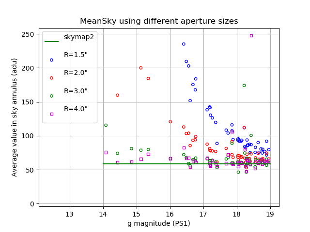
MeanSky Average value in sky annulus (adu)
Npix Number of pixels in aperture
Fpeak Peak Flux (adu) including BKG
Mtype Aperture type (1=circle,2=box,3=ellipse)
g g magnitude (PS1)
r r magnitude (PS1)
i i magnitude (PS1)
B B magnitude (PS1, transformed)
V V magnitude (PS1, transformed)
R R magnitude (PS1, transformed)
dRA_arcsec RA residual (arcseconds)
dDEC_arcsec DEC residual (arcseconds)
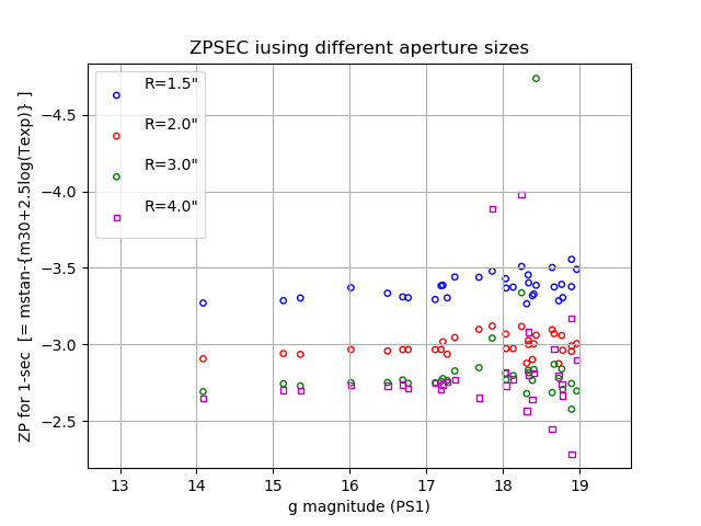
ZPSEC ZP for 1-sec [= mstan-{m30+2.5log(Texp)} ]
magI instrumental magnitude [= m30+2.5log(Texp) ]
g-r Standard Color = g-r
First, I want to be able to take two such ZP files, for two different aperture sizes,
and plot the difference in Mag30 against soemthing like g or MeanSky. The sources in these
two files should be matched, so a general table routine is worth developing for this.
However, a simpler approach could be to use my table file system as it is. I simply use
use multiple phot2 runs to produce ZP tables that use progressively larger aperture
radius values. I then plot ZP vs. g for each of these table file sets into one plot.
Lat night I revised the phot2 code so that I can now record the ZP data files with unique
names. So I'll generate some files and then make a combined plot with each set plotted with
a different color. I am now using the file apphot.config to set values of r apphot, etc...
In this exercise I am changing the apertur radius for each ZP* sest
% cat apphot.config
radarcsec 1.5
NumPixMin   8
Sradarc    3.0

To process each set I use:        % phot2 20191022T025524.2_acm_sci.fits -t
To gather installed header info:  % gethead 20191022T025524.2_acm_sci.fits ZPSEC ZPERR NUMZP SKYSB SKYSBERR  NUMBOX

 set   rad   ZPSEC  ZPERR  NUMZP    SKYSB   SKYSBERR  NUMBOX
ZP1   1.5   -3.3759 0.0137  32      20.1870  0.1470     29
ZP2   2.0   -2.9938 0.0118  32      21.1150  0.0730     29
ZP2   3.0   -2.7901 0.0230  30      21.5730  0.0360     30
ZP4   4.0   -2.8193 0.0606  29      21.5670  0.0670     30

To make a summary plot, I want to plot ZPSEC on the Y axis and g on the X axis.

1) Make the first plot
    Generic_Points N       (use "mpl" to see differnt symbols, colors, etc...)
    xyplotter_auto 20191022T025524.2_acm_sci_ZP1 g ZPSEC 1 N
2) Edit List.1 and Axes.1
3)  xyplotter List.1 Axes.1 N            # final plot
Using this List.1,Axes.1 template I could then easily create a simialr pairs of
files to pot the MeanSky values in a similar way.
The plots above illustrate that using all of the points collected with
photometry from a randomly selected aperture size will introduce systematics
errors. Moreover, we really want points from different magnitude ranges for
the two quantities: we want ZP values from the bright stars, and sky values from
the faint stars. Moreover, the sky value derived from annular measures in the
area of stars may not be the best way to go here. I developed
a skymap routine (skymap2) that derives an
independed sky value using the reults from a previously run image_catalogs to remove
teh effects of dicrete sources in the image. The green line in this plot indicates the
mean sky value from this routine. It is clearly superior to the annulus values derived from
the apphot code.