Last year about this time (Spring 2018) I reduced a lot of acm image sets.
The process of deriving photometric zeropoints got very convoluted and
the endpoint documentation was sparse and hard to follow. The primary high-level
routine I used here was usno_photcal.
The documentation in that links privides info on how I used mido photometry
and the USNO magnitudes. Where things go confusion was ehne I made two
big changes: 91) I began using image and file versions from ./local_red, and
(2) I started using PS1 gri photometry grabbed via a web page interface.
Some new developments over the past year have lead me to once again reorganize
the software for ths process:
- I have better, more general, interactive cursor tools for cleaning the data.
- I have a command line method (ps1_cdfp) for gather the griBVR data
In this document I discuss the process of using
mido photometry gathered interactively with the
ds9_imstats code to derive a mean ZP value for
a single input FITS image. For now I will side-setp the notion of running different
pgases of the job on sets of images and just concentrate on establishing and easy-to-use
tool. Finally, you can read a a good set of
notes that demonstrate and validate the mido approach for deriving ZP.
With a FITS image that has a good WCS calibration in the header, the problem
of deriving a phtometric calibrayion (i.e. for mag = ZP - 2.5log(Flux) we
want to determne the value of ZP) should be as simple as:
- Compute instrument magnitudes (magI) for sources on the image
- Query a catalog like PANSTARRS (PS1) to get standard magnitudes (magS)
in the visinity of our image
- Positionally cross-match these two catalogs and compute
ZP = magI - magS for eavery available source
- Reject bad points and compute a mean value and error for ZP.
I have a wcs-calibrated image = 20190217T122456.6_acm_sci.fits
Here are some steps to a ZP value:
% ds9_imstats 20190217T122456.6_acm_sci.fits N # compute mags from CCD
% ps1_cdfp 20190217T122456.6_acm_sci.fits N # gather PS1 standard mags
% cdfpmatI.sh 20190217T122456.6_acm_sci.cdfp ps1.cdfp 2.0 # cross-match the two cdfp files above
% table_checker cdfpmatI N # make a parlab file
% xyplotter_auto cdfpmatI q q 10 N # make plot(s)
I could:
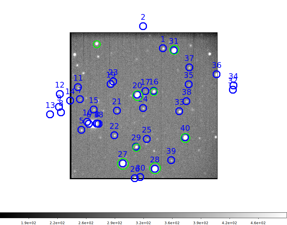
ds9_open 1000 1000
ds9_view_markII 20190217T122456.6_acm_sci.fits zscale n 1 A
(Note: THis plots the markers in 20190217T122456.6_acm_sci.reg)
Then I manually plot: ps1.cdfp.reg
See: zp_example_1.png
What is the filter name?
% image_filter 20190217T122456.6_acm_sci.fits N
i`