 |
| The example 1 plot after the matplotlib show() routine runs. The xyplotter file is really running a python code named pxy_SM_plot.py (which you can read about in my Big List of codes). |
You can use the link here to grab the Ex1 tar file. After you have downloaded the tar file:
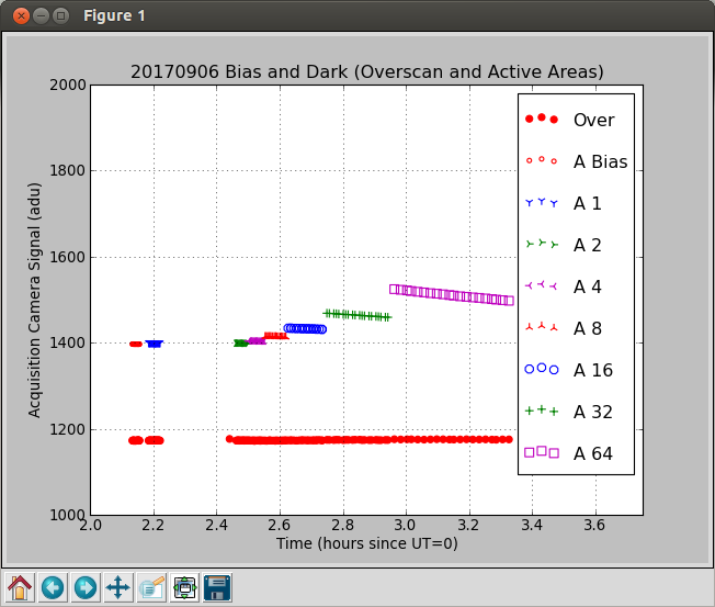
% cp ~sco/Downloads/Ex1.tar .       # Use whatever path you need.
% tar xvf Ex1.tar
% cd Ex1
% cp S/* .
% ls
Axes	   d1.params  d1.table	d32.table  d64.table  dB.table	List.all
d16.table  d1.parlab  d2.table	d4.table   d8.table   dO.table	S/

% xyplotter List.all Axes N
Title = 20170906 Bias and Dark (Overscan and Active Areas)
X: 2.0 3.75      Xtitle = Time (hours since UT=0)
Y: 1000 2000      Ytitle = Acquisition Camera Signal (adu)

To see the plot:
pxy_SM_plot.py STYLE 2.0 3.75 1000 2000 SHOW

View plot now? (Y/N)Y
After you answer "Y" above, then you'll see the plot appear using the matplotlib show() routine. You can adjust the scaling and placement of the data, make a hard copy, etxc... The figure below shows what you should see:
|
| The example 1 plot after the matplotlib show() routine runs. The xyplotter file is really running a python code named pxy_SM_plot.py (which you can read about in my Big List of codes). |
The files in the sample directory are mostly table files. The only essential part of a table file is the *.table file. Here is a sample of the files used here that were compiled using multiple runs of the fits_review routine:
% cat d1.table

# Col01: image number
# Col02: image name
# Col03: object card value
# Col04: filter name
# Col05: RA in sexigecimal format
# Col06: DEC in sexigecimal format
# Col07: structure azimuth
# Col08: parallactic angle
# Col09: wcs presence
# Col10: image source
# Col11: time in dayas since Jan1UT=0
# Col12: time in hours since UT=0
# Col13: signal in bias area (adu)
# Col14: signal in active area (adu)
# Col15: exptime in seconds
# Col16: flux (adu/sec) above bias
# Col17: mean error in flux
# data
1 20170906T021054.8_acm_sci ___ i` 01:13:04.604880 +65:36:09.864000 0.002117 0.004408 Y acm 248.091156 2.18774 1172.6884 1399.5804 227.0091 1 227.009100
2 20170906T021059.5_acm_sci ___ i` 01:13:04.916160 +65:36:09.745200 0.002117 0.004408 Y acm 248.091232 2.18955 1172.8101 1399.5564 226.9518 1 226.951800
3 20170906T021104.1_acm_sci ___ i` 01:13:05.227440 +65:36:09.630000 0.002117 0.004408 Y acm 248.091034 2.18491 1172.3223 1399.4897 226.9955 1 226.995500
4 20170906T021108.8_acm_sci ___ i` 01:13:05.538720 +65:36:09.514800 0.002117 0.004408 Y acm 248.091110 2.18672 1172.9232 1399.6877 227.0539 1 227.053900
5 20170906T021113.4_acm_sci ___ i` 01:13:05.836560 +65:36:09.403200 0.002117 0.004408 Y acm 248.091187 2.18849 1172.8722 1399.5879 226.9421 1 226.942100
6 20170906T021118.1_acm_sci ___ i` 01:13:06.147840 +65:36:09.288000 0.002117 0.004408 Y acm 248.091263 2.19029 1172.8505 1399.5830 226.9458 1 226.945800
7 20170906T021122.7_acm_sci ___ i` 01:13:06.459120 +65:36:09.172800 0.002117 0.004408 Y acm 248.091339 2.19206 1172.6592 1399.5503 226.9690 1 226.969000
8 20170906T021127.3_acm_sci ___ i` 01:13:06.770400 +65:36:09.057600 0.002117 0.004408 Y acm 248.091415 2.19383 1172.8846 1399.5699 226.9350 1 226.935000
9 20170906T021132.0_acm_sci ___ i` 01:13:07.081440 +65:36:08.942400 0.002117 0.004408 Y acm 248.091492 2.19564 1172.8358 1399.4679 226.8533 1 226.853300
10 20170906T021136.6_acm_sci ___ i` 01:13:07.392960 +65:36:08.823600 0.002117 0.004408 Y acm 248.091553 2.19741 1172.8313 1399.4053 226.7877 1 226.787700
11 20170906T021141.3_acm_sci ___ i` 01:13:07.70400 +65:36:08.708400 0.002117 0.004408 Y acm 248.091629 2.19922 1172.6782 1399.3777 226.7746 1 226.774600
12 20170906T021145.9_acm_sci ___ i` 01:13:08.015280 +65:36:08.593200 0.002117 0.004408 Y acm 248.091705 2.20099 1172.3564 1399.4358 226.9464 1 226.946400
13 20170906T021150.6_acm_sci ___ i` 01:13:08.326560 +65:36:08.481600 0.002117 0.004408 Y acm 248.091782 2.20280 1173.0643 1399.3932 225.9452 1 225.945200
14 20170906T021155.3_acm_sci ___ i` 01:13:08.637840 +65:36:08.362800 0.002117 0.004408 Y acm 248.091858 2.20460 1172.8717 1399.3685 226.7629 1 226.762900
15 20170906T021159.9_acm_sci ___ i` 01:13:08.949120 +65:36:08.247600 0.002117 0.004408 Y acm 248.091934 2.20637 1172.4292 1399.3552 226.8556 1 226.855600
16 20170906T021204.5_acm_sci ___ i` 01:13:09.260400 +65:36:08.136000 0.002117 0.004408 Y acm 248.091736 2.20173 1172.8682 1399.5303 226.9226 1 226.922600
17 20170906T021209.2_acm_sci ___ i` 01:13:09.571680 +65:36:08.017200 0.002117 0.004408 Y acm 248.091812 2.20354 1172.5969 1399.3293 226.7527 1 226.752700
18 20170906T021213.9_acm_sci ___ i` 01:13:09.882960 +65:36:07.902000 0.002117 0.004408 Y acm 248.091888 2.20535 1172.9689 1399.4453 226.8151 1 226.815100
19 20170906T021218.5_acm_sci ___ i` 01:13:10.194240 +65:36:07.783200 0.002117 0.004408 Y acm 248.091965 2.20712 1173.0444 1399.4113 225.9697 1 225.969700
20 20170906T021223.2_acm_sci ___ i` 01:13:10.505520 +65:36:07.671600 0.002117 0.004408 Y acm 248.092041 2.20892 1173.0453 1399.3038 225.8610 1 225.861000
21 20170906T021227.8_acm_sci ___ i` 01:13:10.816800 +65:36:07.556400 0.002117 0.004408 Y acm 248.092117 2.21069 1172.6267 1399.2246 226.6286 1 226.628600
22 20170906T021232.4_acm_sci ___ i` 01:13:11.128080 +65:36:07.441200 0.002117 0.004408 Y acm 248.092178 2.21246 1172.8282 1399.3958 226.8018 1 226.801800
23 20170906T021237.1_acm_sci ___ i` 01:13:11.439360 +65:36:07.322400 0.002117 0.004408 Y acm 248.092255 2.21427 1173.4150 1399.3811 225.9047 1 225.904700
24 20170906T021241.7_acm_sci ___ i` 01:13:11.750640 +65:36:07.207200 0.002117 0.004408 Y acm 248.092331 2.21604 1172.8212 1399.3511 226.7411 1 226.741100
25 20170906T021246.4_acm_sci ___ i` 01:13:12.048480 +65:36:07.095600 0.002117 0.004408 Y acm 248.092407 2.21785 1173.4043 1399.3923 225.8988 1 225.898800
26 20170906T021251.1_acm_sci ___ i` 01:13:12.373200 +65:36:06.973200 0.002117 0.004408 Y acm 248.092484 2.21965 1172.4883 1399.1281 226.6314 1 226.631400
27 20170906T021255.7_acm_sci ___ i` 01:13:12.684480 +65:36:06.861600 0.002117 0.004408 Y acm 248.092560 2.22142 1172.4528 1399.2069 226.7122 1 226.712200
This file is not teribbly easy to read, but I have a lot of tools to read and cutup such files. Some of these tool take advantage of supplemental files like these:
% cat d1.params
imgnum
fitsname
object
filter
RAsex
DECsex
AZ
parang
wcsp
imgtype
days
hours
bias
signal
exptime
flux
fluxerr

% cat d1.parlab
imgnum     Image number
fitsname   Name of FITS image
object     Object Name
filter     Filter
RAsex      RA (J2000.0)
DECsex     DEC (J2000.0)
AZ         HET Structure Azimuth (degrees)
parang     HET Parallactic Angle (degrees)
wcsp       WCS presence
imgtype    Image Source
days       Time (days since Jan1 UT=0)
hours      Time (hours since UT=0)
bias       Bias (adu)
signal     Signal (adu) in active area
exptime    Exposure time (seconds)
flux       Flux (ADU/sec) above bias
fluxerr    Flux error
I have only included the params and parlab files for the d1 table file. You could run just the d1 data through xyplotter using a very simple command like:
% xyplotter_auto d1 hours signal 1You can read about xyplotter_auto. It will handle building the Axis and List files. Then you can add more lines to the List file to add more data sets to your plot. Let's take a final look at the List.1 file in our example:
% cat List.all
dO.table   12 13 0 0  point       r o 30   Over
dB.table   12 14 0 0  pointopen   r . 50   A Bias
d1.table   12 14 0 0  pointopen   b 1 50   A 1
d2.table   12 14 0 0  pointopen   g 2 50   A 2
d4.table   12 14 0 0  pointopen   m 3 50   A 4
d8.table   12 14 0 0  pointopen   r 4 50   A 8
d16.table  12 14 0 0  pointopen   b 8 50   A 16
d32.table  12 14 0 0  pointopen   g + 50   A 32
d64.table  12 14 0 0  pointopen   m s 50   A 64
The contents of these lines are explained elsewhere, but a brief reminder is given here:
column   1  = name of the table file to get X,Y data from
columns 2-5 = column numbers of X,Y,Xerr,Yerr
column   6  = type of marker to plot
column   7  = color symbol
column   8  = plot symbol
column   9  = symbol size
column  10  = name of data set for plot legend