Here I am concerned with gathering FITS image header card information into a table file. The primary goal of this exercise is to assemble sky surface brightness values (measured and predicted) and plot them against each other. Also, I wanted to plot each point with a symbol that would indicate the photometric system (i.e. the filter) of each estimate. I had a collection of calibrated acm images with useful information in the FITS headers (you can read about how this image collection was established).

 

I perform (and record) this work in: 
$scohtm/scocodes/munge/ex2_acm/work

I make a list of images: 
% ls -1 /home/sco/acm_reduced/acm/20*fits >list.0 
% head -5 list.0 
/home/sco/acm_reduced/acm/20180114T013423.4_acm_sci_proc.fits
/home/sco/acm_reduced/acm/20180114T013510.1_acm_sci_proc.fits
/home/sco/acm_reduced/acm/20180114T043706.9_acm_sci_proc.fits
/home/sco/acm_reduced/acm/20180114T060057.5_acm_sci_proc.fits
/home/sco/acm_reduced/acm/20180114T071835.6_acm_sci_proc.fits

I make a file that specifies the cards I want to pull:
% cat P.list 
SKYSB       Measured acm Sky Surface Brightness (mag/sq.arcsec)  
MILLUM      Percentage Moon Illumination  
PHIMOON     Angular Separation to Mooon (degrees) 
VSKYSB      Predicted V Sky Surface Brightness (mag/sq.arcsec)  
PSYSNAME    Phtometric system (Filter) 

To make the table file
% fits2table list.0 P.list Data1 N 
% ls 
Data1.params  Data1.parlab  Data1.table  list.0  P.list  S/

# I manually build the following file to specify what I want from the headers.
% cat Data1.parlab 
IMNAME  Name of FITS Image  
SKYSB   Measured acm Sky Surface Brightness (mag/sq.arcsec) 
MILLUM   Percentage Moon Illumination 
PHIMOON   Angular Separation to Mooon (degrees) 
VSKYSB   Predicted V Sky Surface Brightness (mag/sq.arcsec) 
PSYSNAME   Phtometric system (Filter) 

% cat Data1.params
IMNAME
SKYSB  
MILLUM  
PHIMOON  
VSKYSB  
PSYSNAME  

% head -12 Data1.table 
# Col1: ImageName
# Col2: SKYSB   Measured acm Sky Surface Brightness (mag/sq.arcsec)
# Col3: MILLUM   Percentage Moon Illumination
# Col4: PHIMOON   Angular Separation to Mooon (degrees)
# Col5: VSKYSB   Predicted V Sky Surface Brightness (mag/sq.arcsec)
# Col6: PSYSNAME   Phtometric system (Filter)
# data
20180114T013423.4_acm_sci_proc.fits 20.91236 -99.000 -99.000000 21.900000 r
20180114T013510.1_acm_sci_proc.fits -99.00000 -99.000 -99.000000 21.900000 B
20180114T043706.9_acm_sci_proc.fits 21.17308 -99.000 -99.000000 21.900000 r
20180114T060057.5_acm_sci_proc.fits 21.02327 -99.000 -99.000000 21.900000 r
20180114T071835.6_acm_sci_proc.fits 21.14280 -99.000 -99.000000 21.900000 r

To make a mask file that establishes the g images
% table_text_mask Data1 PSYSNAME g mask1 
% head -5 mask1 
N
N
N
N
N
% tail -5 mask1
Y
Y
Y
Y
Y

To make a new table with a mask file
% get_table_rows Data1 mask1 filter_g 
% ls
Data1.params  Data1.parlab  Data1.table  filter_g.params  filter_g.parlab  filter_g.table  list.0  mask1  P.list  S/
% head -12 filter_g.table
# Col1: ImageName
# Col2: SKYSB   Measured acm Sky Surface Brightness (mag/sq.arcsec)
# Col3: MILLUM   Percentage Moon Illumination
# Col4: PHIMOON   Angular Separation to Mooon (degrees)
# Col5: VSKYSB   Predicted V Sky Surface Brightness (mag/sq.arcsec)
# Col6: PSYSNAME   Phtometric system (Filter)
# data
20180114T095949.1_acm_sci_proc.fits 22.45699 -99.000 -99.000000 21.900000 g
20180114T100256.3_acm_sci_proc.fits 22.43568 -99.000 -99.000000 21.900000 g
20180114T103619.2_acm_sci_proc.fits 22.52900 -99.000 -99.000000 21.900000 g
20180114T110845.8_acm_sci_proc.fits 22.35180 -99.000 -99.000000 21.900000 g
20180114T113214.6_acm_sci_proc.fits 21.96765 8.500 57.048183 21.632000 g

Note that wuth our use of the get_table_rows script, we have now created a table of information that contains only data for the g-band images. This new table file with a basename of "filter_g" can be used to make a plot for g data only.

 

% xyplotter_auto filter_g VSKYSB SKYSB 1 
Enter plot title:acm g image data 
Plot a point (P) or a line (L): P 

Title = acm g image data 
X: 17.04500 21.90000      Xtitle = Predicted V Sky Surface Brightness (mag/sq.arcsec)  
Y: 16.34590 22.52900      Ytitle = Measured acm Sky Surface Brightness (mag/sq.arcsec)  

To see the plot: 
pxy_SM_plot.py STYLE 17.04500 21.90000 16.34590 22.52900 SHOW

View plot now? (Y/N)Y 
Plotting: XY.plot.1

Number of points = 53

% ls
Axes.1	      Data1.parlab  figure_1.png     filter_g.parlab  list.0  mask1   S/
Data1.params  Data1.table   filter_g.params  filter_g.table   List.1  P.list

I change the legend name and the plot symbol:
% cat List.1 
filter_g.table   5 2 0 0   point g o 40  g  

# I make the new plot 
% xyplotter List.1 Axes.1 

# Following the examples above I now make tables of B and r data and 
# prepare a new multi-data plot 

NOTE:  I use the "mls" alias to remember point type sna attributres:
% mpl 

# Get the r data 
% table_text_mask Data1 PSYSNAME r mask2
% get_table_rows Data1 mask2 filter_r  

# Get the B data 
% table_text_mask Data1 PSYSNAME B mask3 
% get_table_rows Data1 mask3 filter_B 
 
# I manually made the Table for my unity line:  filter_LINE.table,parlab

You can read a more detailed discussion of xyplotter_auto and see different exmaples of making plots. Below is the final plot I made.

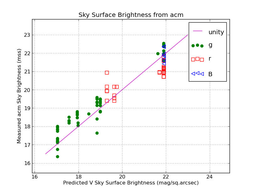The sky surface brightness values from acm images taken in the B, g, and r filters. Here are the files and command I used to make this: % cat ../work/Axes.1 Sky Surface Brightness from acm 17.04500 21.90000 Predicted V Sky Surface Brightness (mag/sq.arcsec) 16.34590 22.52900 Measured acm Sky Brightness (mss) % cat ../work/List.1 filter_g.table 5 2 0 0 point g o 40 g filter_r.table 5 2 0 0 pointopen r s 60 r filter_B.table 5 2 0 0 pointopen b < 60 B filter_LINE.table 5 2 0 0 line m - 60 unity % xyplotter List.1 Axes.1