A revised and experimental version of ds9_profiles. Actually, the original ds9_profiles was experimental also. It was intended to verify and visualize the source code need to compute a radial intensity profile. As the name implies we can use three type of ds9 regions to define and measure an aperture that is: an ellipse, a circle, a box. The box region can be used to measure fixed (constant) sky estimates for every aperture meausered in a run. The boses can also be used to measure the X or Y marginal distrubutions needed to, for instance, measure a spectral line profile. There are some fancy-pants routines for doing things like setting an ellipse for the center or a galaxy and also one for the outer isophote of the galaxy.

 
%  ds9_profiles_x --help  
usage: ds9_profiles_x a.fits [-v] [-h] [-fp] [-s ] [-m ] 
Additional options: 
     -v         = print verbose comments and run in debug mode 
     -h         = show a help file and then exit 
     -s, --sky  = sky method (FIXED SKY,LOCAL_SKY)  
     -m, --maxk = pixel exclsuion mask (can be none)  

 
%  ds9_profiles_x 20191018T084633.3_acm_sci.fits -s FIXED_SKY -v   

Note that becasue O use "-s FIXED_SKY" I will set some sky boxed. I use the "-v" flag 
becasue I want to leave the shit-ton of peripheral files made in the run so that I can 
show some important ones below. Whn you use the "-v" flahg, this routine will be extremely 
verbose and you will hav to respond to many questions like "Enter any key to continue:". 
But, all in good fun.  

The most important file from the ds9 run is "profpars.out". This will contain the infomation 
needed for measuring the profile of each aperture (one aperture per line, each aperture 
defined by a ds9 region): 

% cat profpars.out_explain 
# Output columns from profpars (using midodata.2)
Col01 = X center, pixels (from centroid)
Col02 = Y center, pixels (from centroid)
Col03 = semi-major axis length in pixels  
Col04 = b/a axis ratio
Col05 = position angle (degrees) of major axis 
Col06 = local background measured in local annulus 
Col07 = mean bkg (signal per pixel) from BOX regions
Col08 = mean error of mean bkg (BOX regions)
Col09 = id, line number in regions file 

% cat profpars.out 
     413.900      301.950       34.000  1.00000    0.000     482.8040     479.3014       3.0678     1

Note that column 6 has the local sky value measured in the local annulus used by mido.sh. 
Column 7 is the mean sky value measurede with the 3 sky boxes I set. 

After the run for our simple aperture is completer, we wee: 
% ls 
20191018T084633.3_acm_sci.cdfp	20191018T084633.3_acm_sci.info
20191018T084633.3_acm_sci.fits	20191018T084633.3_acm_sci.reg	ap_1/		

The profile infomation for our one aperture is in two table files in ./ap_1:
% ls ap_1 
profile_gcurve_kfit.parlab  profile_gcurve.parlab  profile_pnts.limits	profile_pnts.parlab
profile_gcurve_kfit.table   profile_gcurve.table   profile_pnts.log	profile_pnts.table
profile_gcurve.log	    profile_pnts.header    profile_pnts.out

profile_pnts:  The individual (pixel) profile points 
% cat profile_pnts.parlab 
rad          Radius in units of pixels 
I-Isky       Signal (above background) in ADU 
i            x pixel position in full image  
j            y pixel position in full image  (pixels) 
I            Signal (adu)    
Isky         Background Signal (adu) 
rad^0.25     Radius**0.25 (Radius in pixels) 
log(I-Isky)  log10 of Signal(adu) above background

% table_checker profile_pnts N
3622 8 
 

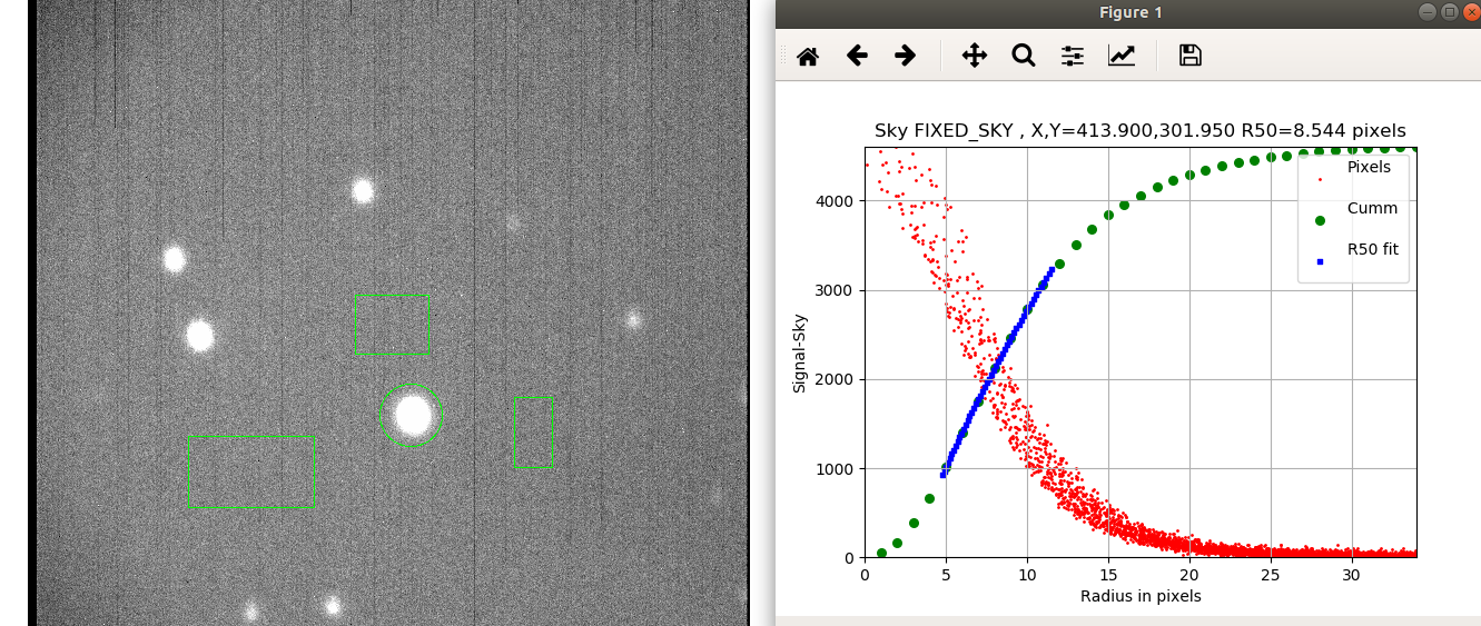
gcurve_kfit:   The cuumulative signal curve. 
% cat profile_gcurve_kfit.parlab 
rad    Radius in pixel units 
k      Fraction of total Signal 

% table_checker profile_gcurve_kfit N
50 2 

 
 

The large-text blue info shows why this is a demo code! The profile file is huge, and this is only for a star. A large galaxy in the image would be insanely large. What we need to go along with our demo code is a routine that runs much of the computational source code of ds9_profiles_x, but holds this profile information in memeroy. We could parameterize of fit the profile with something beyond a simple R50 value and we could fo it for many apertureds on an image.

An example of a ds9_profiles_x run on a processed acm image (left) where we have marked a star with a circle region and 3 box regions to use for ccomputing a fixed sky level. The resulting profile is shown in the matplotlib show() window on the right. Each pixel in the radial profile is represented by a red dot. The green circles represnt the signal groth curve (the integral of the radial profile) and would typically be used to compite a total signal. We can use this curcve to identify the radius of the aperture that would contain half of the total signal (often called the half-light radius). The blue dots represents the curve used for thsi purpose, andt the hal-light radius, in pixel units, is printed in the plot title (the value R50, for the Radius of the aperture containing 50% of the total integrated flux).