combine_waversols
Updated: Oct03,2020
Combine spectral feature sets collected from lmap_markII
runs and derive a linear wavelength solution.
%
% combine_waversols -h

usage: combine_waversols 056LL [-v] [-h] [-c]
arg1 = device name (ifu+amp, e.g. 056LU)
Additional options:
  -h = just show usage message
  -v = run in verbose/debug mode
  -c = just run the cleanup function

See examples in:   /home/sco/LRS2_wavesols/20200529-30/

The basic rsults are stored in a local subdirectory named Plot_1.
Here is an example:
% pwd
/home/sco/LRS2_wavesols/20200529-30/uv_old/056LU/Plot_1
% ls
056LU.solution	    curve_runner.results       line.clcf_rstats.resids.1     line.fitcurve.2	 line.out.Last
Axes.1		    line.clcf_rstats.out.1     line.clcf_rstats.resids.2     line.fitcurve.Last  List.1
clcf_rstats.out     line.clcf_rstats.out.2     line.clcf_rstats.resids.Last  line.out.1
clcf_rstats.resids  line.clcf_rstats.out.Last  line.fitcurve.1		     line.out.2
The 056LU.solution file contains the linear solution as well as a copy of the Big2.table file.
The Axes.1 and List.1 files can be used to replot the wavelength solution using
xyplotter.
 |
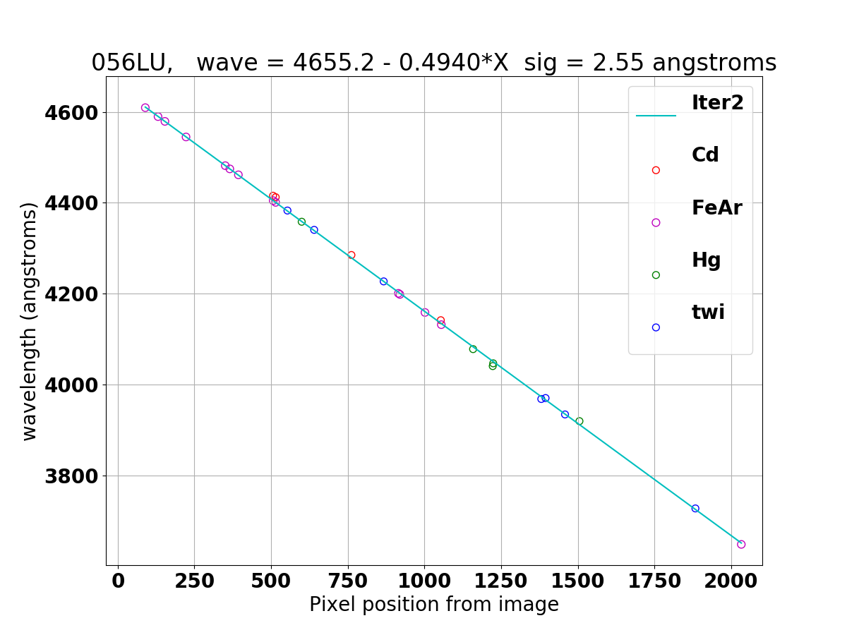 |
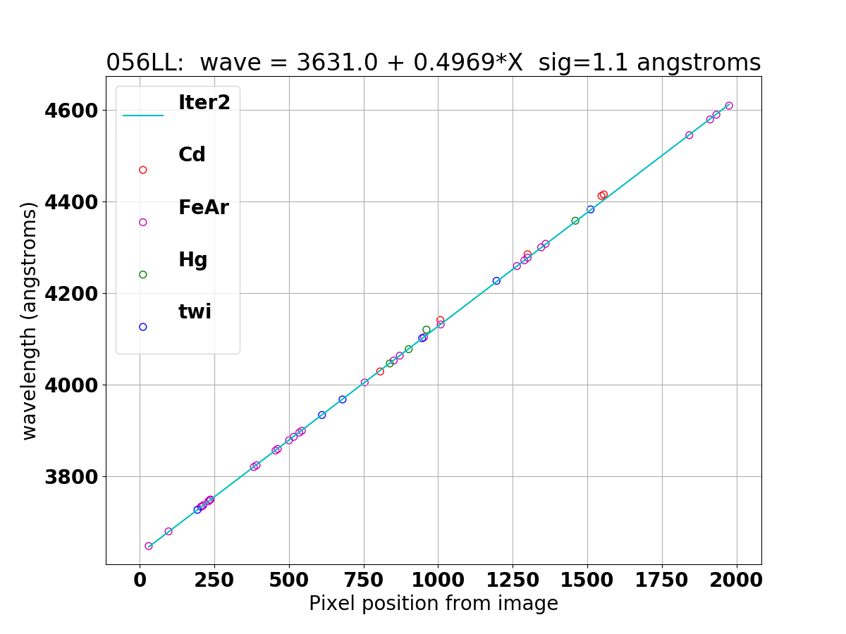
Wavelength solution for 056LL (top) and 056LU (bottom) derived with combine_waversols.
% xyplotter List.1 Axes.1 N

% cat List.1
20200529T231708.8_056LU_cmp_uv_Cd_wsol.table    1 2 0 0 pointopen  r o 50 Cd
20200529T231708.8_056LU_cmp_uv_FeAr_wsol.table  1 2 0 0 pointopen  m o 60 FeAr
20200529T232458.0_056LU_cmp_uv_Hg_wsol.table    1 2 0 0 pointopen  g o 50 Hg
20200530T020734.3_056LU_twi_uv_ALL_wsol.table   1 2 0 0 pointopen  b o 50 twi
line.fitcurve.2 1 2 0 0   line  c - 10  Iter2

% cat Axes.1
056LU,   wave = 4655.2 - 0.4940*X  sig = 2.55 angstroms
  89.86000 2033.01000 Pixel position from image
  3647.84200 4609.56700 wavelength (angstroms)
|
It is useful to show a typical directory structure before we run combine_waversols:
% pwd
/home/sco/LRS2_wavesols/20200529-30/uv/056LU_wsol

% ls
20200529T231708.8_056LU_cmp.fits		 20200529T232458.0_056LU_cmp.Image.Info
20200529T231708.8_056LU_cmp.Image.Info		 20200529T232458.0_056LU_cmp_uv_Hg_wsol.curve
20200529T231708.8_056LU_cmp_uv_FeAr_wsol.curve	 20200529T232458.0_056LU_cmp_uv_Hg_wsol.parlab
20200529T231708.8_056LU_cmp_uv_FeAr_wsol.parlab  20200529T232458.0_056LU_cmp_uv_Hg_wsol.table
20200529T231708.8_056LU_cmp_uv_FeAr_wsol.table	 20200530T020734.3_056LU_twi.fits
20200529T232057.1_056LU_cmp.fits		 20200530T020734.3_056LU_twi.Image.Info
20200529T232057.1_056LU_cmp.Image.Info		 20200530T020734.3_056LU_twi_uv_ALL_wsol.curve
20200529T232057.1_056LU_cmp_uv_Hg_wsol.curve	 20200530T020734.3_056LU_twi_uv_ALL_wsol.parlab
20200529T232057.1_056LU_cmp_uv_Hg_wsol.parlab	 20200530T020734.3_056LU_twi_uv_ALL_wsol.table
20200529T232057.1_056LU_cmp_uv_Hg_wsol.table	 S/
20200529T232458.0_056LU_cmp.fits
Theses are the bias-subtracted FITS files and the line identification files
deposited in the devive-specific directory (056UL_wsol) by the runs of lmap_markII
(with the "-w" flag in use). The ./S subdirectory is just a place where I store the table
files. I also run the "getrc" and "Generic_Points" scripts there to produce plot parameter
files that make easier to run xyplotter_auto.
After I run combine_waversols we'll some more table file
that combine all of the spectral lines, and a subdirectory that will contain the
files used by xyplotter that we do not want
to be overwritten during the next reduction step.
% combine_waversols 056LU

% ls
20200529T231708.8_056LU_cmp.fits		 20200529T232458.0_056LU_cmp.fits		 Big2.parlab
20200529T231708.8_056LU_cmp.Image.Info		 20200529T232458.0_056LU_cmp.Image.Info		 Big2.table
20200529T231708.8_056LU_cmp_uv_FeAr_wsol.curve	 20200529T232458.0_056LU_cmp_uv_Hg_wsol.curve	 Big.parlab
20200529T231708.8_056LU_cmp_uv_FeAr_wsol.parlab  20200529T232458.0_056LU_cmp_uv_Hg_wsol.parlab	 Big.table
20200529T231708.8_056LU_cmp_uv_FeAr_wsol.table	 20200529T232458.0_056LU_cmp_uv_Hg_wsol.table	 Figure_1.png
20200529T232057.1_056LU_cmp.fits		 20200530T020734.3_056LU_twi.fits		 matplotlibrc
20200529T232057.1_056LU_cmp.Image.Info		 20200530T020734.3_056LU_twi.Image.Info		 Plot_1/
20200529T232057.1_056LU_cmp_uv_Hg_wsol.curve	 20200530T020734.3_056LU_twi_uv_ALL_wsol.curve	 S/
20200529T232057.1_056LU_cmp_uv_Hg_wsol.parlab	 20200530T020734.3_056LU_twi_uv_ALL_wsol.parlab  xyplotter_auto.pars
20200529T232057.1_056LU_cmp_uv_Hg_wsol.table	 20200530T020734.3_056LU_twi_uv_ALL_wsol.table
Notice that the ./Plot_1/ is created, and this contains the plot files we need to
view a figure showing the wavelenght vs. X position data and the linear fits made to
that data. Another important file in the ./Plot_1 subdireorty is the final wavelength
solution file, in this csae ./Plot_1/056LU.solution.
Back to SCO CODES page