I used the code ts_plot.py to assure that I got the same scale on the X,Y axues of a plot. But waht if I want the data plotted to a specific scale?

1. An experimental code.
2. Compiling and measuring plots.

Here is a simple code that I use to make FIGURES of a different sizes.

 

#!/usr/bin/env python

import argparse as ARGP
parser = ARGP.ArgumentParser()
parser.add_argument("arg1", help="figure width in inches")
parser.add_argument("arg2", help="figure height in inches")
parser.add_argument("-v","--verbose", help="Verbose responses",
                    action="store_true")
args = parser.parse_args()
 
# Setup to read the name of the input file 
width_inch = args.arg1
height_inch = args.arg2

# Numpy is a library for handling arrays (like data points)
import numpy as npsubs

# Pyplot is a module within the matplotlib library for plotting
import matplotlib.pyplot as plt

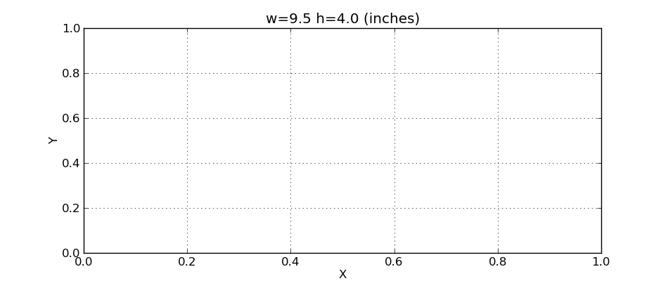
label_main  = "w=%s h=%s (inches)" % (width_inch,height_inch)
label_xaxis = "X" 
label_yaxis = "Y" 

xlo="0.0"
xhi="1.0"
ylo="0.0"
yhi="1.0"

verbo = args.verbose
#print verbo

if args.verbose:
 print "Plot (for sco) title = %s\n" % (label_main),
 print "X-axis title = %s\n" % (label_xaxis),
 print "Y-axis title = %s\n" % (label_yaxis),
 print "X range = %s %s \n" % (xlo, xhi),
 print "Y range = %s %s \n" % (ylo, yhi),

#=========================================================
#plt.axes(aspect=1)
wid = float( width_inch ) 
hei = float( height_inch ) 
plt.figure(figsize=(wid,hei))
#=========================================================

# add some fancy touches 
plt.grid(True) 
#plt.legend() 

xlim1 = float(xlo)  
xlim2 = float(xhi) 
ylim1 = float(ylo) 
ylim2 = float(yhi) 
plt.xlim(xlim1,xlim2)
plt.ylim(ylim1,ylim2)

# label the axes 
plt.title(label_main) 
plt.xlabel(label_xaxis)
plt.ylabel(label_yaxis)

plt.savefig('pxy.png')

#print '\nUse to view your plot:\ndisplay pxy.png\n'

To run this code: 
% prun 9.5 4.0 001
% prun p001.png 

I wanted to understand how to specify the size and scale of a matplotlib.pyplot figure. To make this plot: % prun 9.5 4.0 001 % display p001.png The final plot has a figure size that has a width of 10.25 inches and height of 4.5 inches. The actual size of the X,Y axes (in the display monitor) is a width of 8.0 inches and a height of 3.5 inches.

Using the code in the previous section I made a script to run lots of plot examples using different sizes:

 

% cat BIGRUN 
#
prun 3.0 8.0 001
prun 4.0 7.0 002
prun 5.0 6.0 003
prun 3.0 5.5 004
prun 5.5 4.0 005
prun 6.5 9.0 006
prun 9.5 4.0 007

 

% cat Table.dat 
# col01: name 
$ col02: X input 
$ col02: Y input 
# data 
p001.png   3.00 8.00   2.50  6.75 
p002.png   4.00 7.00   3.50  6.00 
p003.png   5.00 6.00   4.25  5.25 
p004.png   3.00 5.50   2.50  4.75 
p005.png   5.50 4.00   4.50  3.50 
p006.png   6.50 9.00   5.50  7.75 
p007.png   9.50 4.00   8.00  3.50 

 

% xyplotter_prep Table.dat 1
Enter plot title:X data
Enter X,Y column numbers (1 2): 2 4
Enter X,Y error column numbers (0 0): 0 0
Enter X-axis label:X input 
Enter Y-axis label:X monitor width

You are set up to make a plot with Table.dat
Here is the command line to use:
    xyplotter List.1 Axes.1 

% xyplotter List.1 Axes.1

Then I could modify the files List.1 and Axes.1 to get:

% cat List.1
Table.dat   2 4 0 0   point  r o 70   X data 
Table.dat   3 5 0 0   point  b s 70   Y data 
% cat Axes.1
X,Y Sizes in matplotlib.pyplot 
  1.0  12.0    X input 
  0.0  12.0    X monitor width 

I fit both sets of data with a line:
  Size_Monitor =   0.038  +   0.846 * Size_Input 
                  -+0.07    -+0.012 

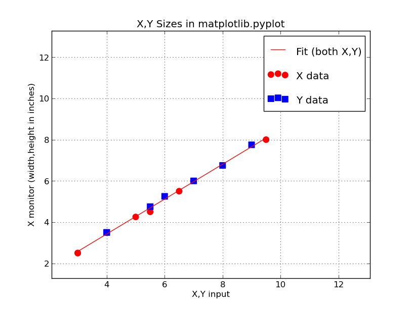The X,Y sizes of sizes I measure on my monitor verses the X,Y sizes I input the matplotlib. I fit both sets of data with a line: Size_Monitor = 0.038 + 0.846 * Size_Input -+0.07 -+0.012 Practical (working) equation: Size_Input = 1.182 * Size_Monitor - 0.045 Hence, if I wanted to make a square that is 6" x 6" I would use: % prun 7.047 7.047 200 % display p200.png At some point I'll measure these plots on paper and derive the same sort of linear fit. For now, I'll use the above relation to set the X,Y sizes on on my plots. Actually, what I want to specify is size on the monitor (or paper print) and then predict the figure size (Size_Input). So the working equation is really the second equation above.