 |
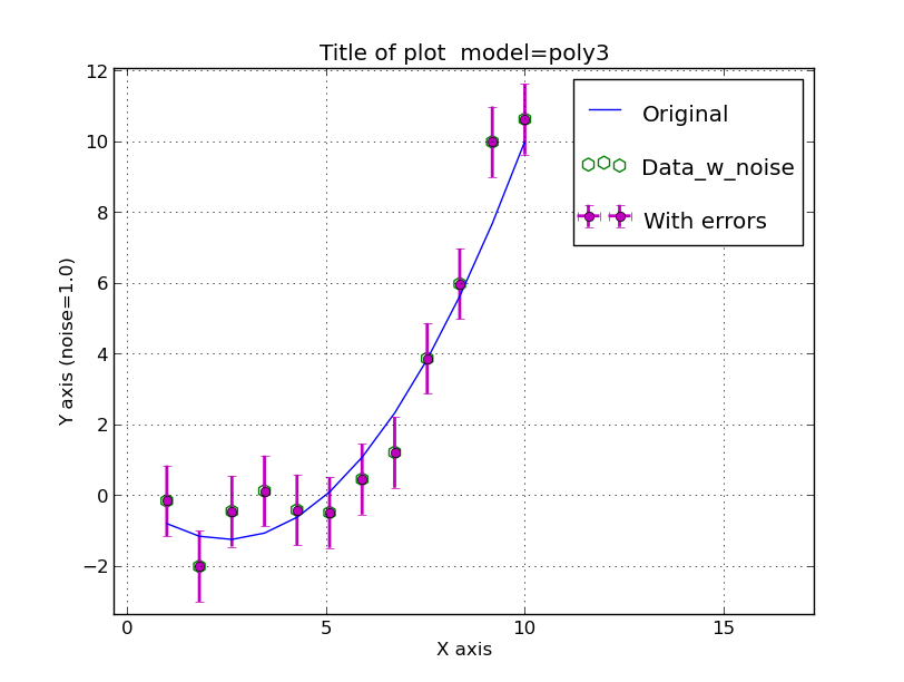
A simple parabola generated with make_fit_data:
% make_fit_data poly3 c.3 12 1 10 0.0 1.0 % cat c.3 0.0 -1.0 0.2 % xyplotter List.1 Axes.1 % pxy_SM_plot.py STYLE 1 10 -2.00875 10.62608 SHOW |
I depart my verbose ways and give a short set of examples of I generate a set of test data, plot it, and fit it.
I use the "make_fit_data" script to generate points on a parabola (curve type = "ploy3"). This script also build the files I need for viewing a plot of the dat points. The package provides instructions that step you trhough the process.
% make_fit_data poly3 c.3 12 1 10 0.0 1.0
No file = c.3
curve,outfile = poly3 c.3
Equation form:   Y = a1 + a2*X + a3*X^2
Ready to read the 3 coefficients.
  Enter coefficient 1: 0.0
  Enter coefficient 2: -1.0
  Enter coefficient 3: 0.2
To plot the data:
xyplotter List.1 Axes.1

% ls
Axes.1	c.3  List.1  Table1.dat

% xyplotter List.1 Axes.1
Title = Title of plot  model=poly3
X: 1 10      Xtitle = X axis
Y: -2.00875 10.62608      Ytitle = Y axis (noise=1.0)
To see the plot:
pxy_SM_plot.py STYLE 1 10 -2.00875 10.62608 SHOW
%
% ls
Axes.1	c.3  List.1  STYLE  Table1.dat	XY.plot.1  XY.plot.2  XY.plot.3
|
A simple parabola generated with make_fit_data:
% make_fit_data poly3 c.3 12 1 10 0.0 1.0 % cat c.3 0.0 -1.0 0.2 % xyplotter List.1 Axes.1 % pxy_SM_plot.py STYLE 1 10 -2.00875 10.62608 SHOW |
Maybe I want to chane up the data set a little before I procedd. In
addition to deomontrating how we'll fit a polynomial to these data, we'll
wan to demo the routine that rejects bad points, so maybe we'll throw
in a really bad point in out test set to make this process clear. Maybe we
want to give the plot some facier titles. I make a few changes to our three
basic files and re-run xyplotter to get the plot below.
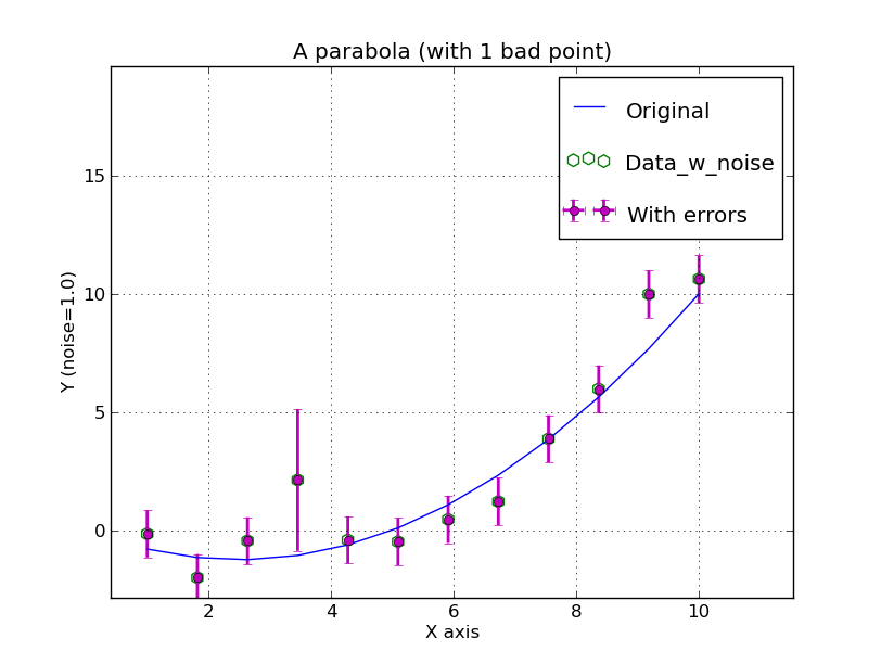 |
Here is our simple parabola exampel witha few changes. I have
added a bad point (the fourth point in the X direction with the larger error
bar), and I have changed the axis labeling. After these changes (to Table1.dat and
Axes.1) I reran "xyplotter" and go my new plot in a few seconds.
% xyplotter List.1 Axes.1

% cat Table1.dat
# Tests data generated with make_fit_data
# func = poly3
# N terms =  3
       0.000000000
      -1.000000000
       0.200000003
# Gaussian noise added to X = 0.0
# Gaussian noise added to X = 1.0
# col01 = X value
# col02 = Y value
# col03 = X value with X noise added
# col04 = X value with Y noise added
# col05 = X error
# col06 = Y error
# data
  1.00000	  -0.80000	      1.0000000	     -0.1567700	  0.0	  1.0
  1.81818	  -1.15702	      1.8181800	     -2.0087500	  0.0	  1.0
  2.63636	  -1.24628	      2.6363599	     -0.4513500	  0.0	  1.0
  3.45455	  -1.06777	      3.4545500	      2.1224700	  0.0	  3.0
  4.27273	  -0.62149	      4.2727299	     -0.4156800	  0.0	  1.0
  5.09091	  0.09256	      5.0909100	     -0.4870900	  0.0	  1.0
  5.90909	  1.07438	      5.9090900	      0.4547501	  0.0	  1.0
  6.72727	  2.32397	      6.7272701	      1.2113901	  0.0	  1.0
  7.54545	  3.84132	      7.5454502	      3.8649700	  0.0	  1.0
  8.36364	  5.62645	      8.3636398	      5.9739299	  0.0	  1.0
  9.18182	  7.67934	      9.1818199	      9.9851093	  0.0	  1.0
  10.00000	  10.00000	     10.0000000	     10.6260796	  0.0	  1.0

% cat Axes.1
A parabola (with 1 bad point)
 -1 14      X axis
 -2  14.0   Y (noise=1.0)

% cat List.1
Table1.dat   3 4 5 6   pointopen   g h 70   Data_w_noise
Table1.dat   1 2 5 6   line        b - 70   Original
Table1.dat   3 4 5 6   errorbar    m o 10   With errors
|
I use the "make_fit_data" script to generate points on a parabola (curve type = "ploy3"). This script also build the files I need for viewing a plot of the dat points. The package provides instructions that step you trhough the process.
% ls
Table1.dat
% curve_fit_prep Table1.dat 3 4 poly3 REJO
# This uses the code clcf_makexy.sh

% ls
head.lines  junk  REJO	Table1.dat  X.dat  Xor	Y.dat  Yor

% curve_fit poly3 X.dat Y.dat 30

% curve_fit_omc Table1.dat 3 4 poly3 REJO
# Now I have:  Xor,Yor,Ycal    (for original set)

% clcf_rstats.sh Yor Ycal REJO 2.5
   12       1.2538463         11         0.7680258
Hence, at the end of this sequence we have 11 unrejected points (with the one bad point now marked in a revised REJO file). We could re-run the sequence and derive a better fit.
The commands above are best run from a simple wrapper script: curve_runner.
% curve_runner 4

The command above (for List.4,Axes.4) will run up to 5 iterations of:
% curve_fit_prep Table1.dat 3 4 poly3 REJO
% curve_fit poly3 X.dat Y.dat 30
% curve_fit_omc Table1.dat 3 4 poly3 REJO
% clcf_rstats.sh Yor Ycal REJO 2.5
A short, highly volatile list of script calls to demos XY operations.
% make_fit_data poly3 c.3 12 1 10 0.0 1.0
# Sample values:  0.0   -1.0   0.2

# If Table1.dat is any real data file:
# xyplotter_prep will set up our files for plotting:
% xyplotter_prep Table1.dat 1
% xyplotter List.1 Axes.1

# Fit and view the data for List.1 and Axes.1:
% curve_runner 1