Evaluating a night of acm images
Last updated: Jan19,2019
This is an early document describing my acm reduction methods. The
software and the descriptions changed a lot as we learned more about the properties
of this camera. I archive this doc now in Feb2019.
The motivation for this document centered around measuring night sky surface brightness
values with the acm. The bias, and to a lesser extent the dark levels, must be subtracted
before we can measure a mean flux level due to the sky signal. Some early numbers from an
analysis of sky frames indicate that if we assume a bias uncertainty of &pm 6 adu (if no
bias fraem are available for a given night) then our sky flux uncertainties will be 11%
and 3% in g,r respecticvely. The derivation of these estimates is described in
a quick first look at g,r sky levels..
- A full end-to-end reduction of a night.
- Published sky brightness measurements.
- A useful set of nights.
- A quick first look with fits_review.
- A survey of multiple nights.
- Summarizing a single night.
- Visually checking a lot of images.
- Obtaining bias and dark frames at the telescope.
- Buildng a master bias frame.
- Buildng a master darkrate frame.
- Initial pipeline processing.
- Install useful WCS solutions.
- Derive and install photometric ZP values. (General)
- A working catalog and image header additions.
- Analysis
- A summary of the image material.
- Appendices: A variety of docs related to acm processing
A full end-to-end reduction of a night.
In a "cart before the horse" approach, I have decided to first present a
sequential description of how I go about reducing a single night of acm data.
The variable nature of the acm instrument has dictated numeroud changes to
this process, and this variation will doubtless continue. Hence, my solution is
to link to a verbose document that outlines the best set of steps that are
currently in use. I'll updat and/or replace this document as the need arises.
The current process is outlined in an
End-to-End Reduction of 20180403.
Published sky brightness measurements.
A big motivator fro this work was to measure night sky surface brightnees values
with the acm using differential photometry from stars in ean acm field. Here
are some wuicky notes.
# Use https://www.google.com/  and search on "dark sky g band sky brightness"

http://www.ctio.noao.edu/noao/node/1218
 *** Lots of good references and these mean values:

U 	22.12 mag arcsec-2
B 	22.82 mag arcsec-2
V 	21.79 mag arcsec-2
R 	21.19 mag arcsec-2
I 	19.85 mag arcsec-2

u 	23.3 mag arcsec-2
g 	22.3 mag arcsec-2
r 	21.4 mag arcsec-2
i 	20.5 mag arcsec-2
There are other papers (de Vaucoleurs and Angione at McD, Violet Taylor at VATT, etcc)
to collect good UBVR stuff, but the numbers above are a good ballpark start.
A useful set of nights.
This document originally dealt with the reduction of a single night. In
practice, many recution problems were encountered and in the end a number of
nights were analyzed. I record information about these nights below.
A valuable night:  20180114     Moon rise at 11:50 UT
  Nearly all of the night was dark (no moon) and clear. I took acm cals
  and a number of acm images on sky associated with LRS2 observations. This
  night should have all we need for dark sky surface brightness measurements.
  Clear at start of night, no further weather notes

A valuable night:  20180115     Moon rise at 12:40 UT
  Took sky brightness data in grB on acm with open cluster NGC2301. Took
  bias and dark frames with scripts, bias=1382 (normal).
  Cirrus at start of night, no further weather notes
A valuable night:  20180116
  Bad weather, no observing. Took extensive bias+dark with stacking by scripts.

A valuable night:  20180206      Moon rise at 6:10UT
  Took acm bias and 5sec darks that appear to be normal. Observed many targets
  with dark time and bright moon time. Should be excellent for sky brightness work.
  Took mainly B,r acm images.
  Notes indicate night clear

A valuable night:  20180402    Moon rise at 2:50UT
  Pointing test night where I took 30-60 stars each night almost all in g. I
  also took bias/dark data sets (which appear to be at normal levels). This
  night had a very bright moon a day or two after full moon. Mostly clear
  in the time range 6:30UT to 10:20UT.
  Some clouds, some clear

A valuable night:  20180403    Moon rise at 3:40UT
  Pointing test nights where I took 30-60 stars each night almost all in g. I
  also took bias/dark data sets (which appear to be at normal levels). Both
  nights had a very bright moon a day or two after full moon.  Clear in early
  part of the night with some clouds around 6:00UT.  Heavy clouds and high
  wind after 8:23UT.
  Some clouds, some clear
Note that I include the night of 20180116, a night of heavy clouds when we made no
on-sky observations. A major obstacle in analyzing acm data for sky surface brightness
analysis involves how best to subtract the bias and dark signals in these images. ON
20180116 we took numerous bias and dark frames to address these issues.
A quick first look with fits_review.
In a given night we'll usually see a wide variety of acm images. Some can be
final (just prior to LRS2 or VIRUS observation) setup images, some are intermediate
sky images taken during focus and telescope position, some may be various types of
calibration images (skyflat, bias, dark, etc...). In some cases the RA logs may help
you navigate the different image types, but a lot of times we just have a directory
full of images. The routine fits_review
is designed to operate on a variety of image types, and I initailly used it here
to evaluate images taken with the HET acquisition camera (acm).
This approach is described here.
Eventually I realized that the acm image data suffers many problems. Poor or incorrect
header information, variable bias and dark signal, and a number of other annoying
trends make a direct approach to reduction impossible. A set of routines that are
specifically built for efficient acm processing were eventually developed.
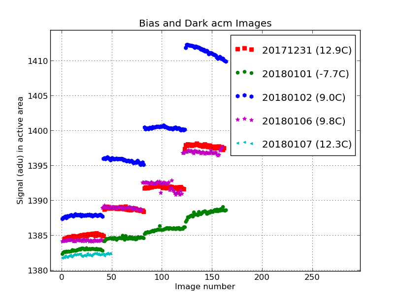
One of the most fundamental problems encountered in acm image analysis is the variable
nature of the bias level. Using the early fits_review analyses I constructed the figures
below that demonstrate this problem.
 |
|
The bias and dark frame signals found in different nights of acm image data. Initially I
thought these values may have a strong temperature dpendence. However, looking at the
temperature values given in the legend we see that this is not strictly true. In this
plot I have the BIAS images hving the lowest images numbers and then I include dark
images with progressively longer integrations times of 5sec, 10sec, and 20sec.
|
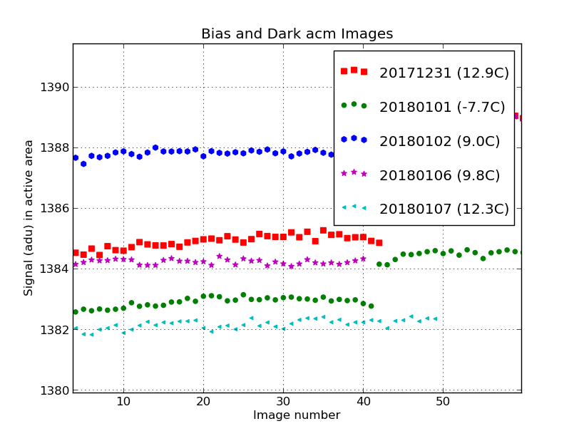
I made a zoomed in version of the above figure to give the reader a clearer
view of the bias variation we encounter among different nights.
 |
|
The bias and dark frame signals found in different nights of acm image data. I
have zoomed in on the bias images to show that for five different nights we
encounter bias levels that range from 1382 adu to 1388 adu. Initially I had hoped
this scatter over 6 adu would be explained by temperature vaiation, but this is not
true. The two lowest values come from the coldest (20180101,green) and one of
the warmest (20180107,cyan) nights. The lesson here is that we'll
need at least a few acm bias frames per night if we are to properly correct for the
mean bias level in acm images from a given night.
|
There has been talk of developing a bais overscan for the acm camera, but this
is in the "when pigs fly" regime.
A survey of multiple nights.
In trying to outline how I would reduce a single nights-worth of acm images I
uncovered a host of problems. To treat many of these required me to inspect
and compare image properties from many nights.
Using fits_review to characterizethe acm images from
a given night is useful. However, problems with variable bias and dark properties necessitated
using many nights of daqta to address these issues. To easily summarize many nights of data
I developed the routine acm_nights. Basically I want
use a file that lists the dates I am interested in, and the location on disk where my date subdirectories
are located (for example, on mcs we usually used /hetdata/data). Here is a brief example:
  # In the file "list.1" I listed 13 nights of interest
% acm_nights list.1 /home/sco/HET_work/acm_nights
Results are written to:    acm.nights_TABLE
20170906     220    23   148    49
20171108     878   573   305     0
20171129      94    60    19    15
20171231     544    42   120   382
20180101     164    40   123     1
20180102     682    41   123   518
20180105     213    40   120    53
20180106     272    40   120   112
20180107     305    62    13   230
20180109     387    41    45   301
20180114     352    12    27   313
20180115     529    11    21   497
20180116     309   224    84     1

The columns are:
Col01:  UT date
Col02:  total number of images
Col03:  number of bias images
Col04:  number of dark images
Col05:  number of "shutter-open" images
Using this approach I could survey in less than a minute the contents of
the 13 nights (as of Jan22,2018) when bias frames were takenfor the acm.
This would have taken considerably longer with separate runs using fits_review.
Summarizing a single night.
Once a night has been selected for reduction, we want to start with a simple
summary of waht images are available.
  # Procedure as of Mar20,2018
 wheredata Y
 acm_list none none
OR
  setenv basedir /home/sco/HET_work/acm_nights    (in BaseDir)
  setenv date 20180206                            (in Date)
  acm_list $date $basedir
This procedure will create lists of images like list.OPEN, list.DARK, and list.BIAS. Some
of this files can be large (hundreds of lines) and not easily used for visual review, etc..
The list.OPEN file is usually very large, and this is the list of images that we
presumably care the moset about (images taken on the sky mostly!).
There are some useful scripts that can be used to divide them furtehr:
% list_split_exptime list.OPEN ListEXP Y   # Divide into lists split by (integer) exposure tie in seconds
% list_split_filter list.OPEN List N       # Divide into lists split by filter name
You can see exmaples of using
list_split_exptime and
list_split_filter.
Visually checking a lot of images.
Sometimes we want to view large numbers of images. Here are some ways
to do this. The images can be marked and the resulting lists of marked
and unmarked images can be used for various tasks.
# Viewing multiple acm images.
 acm_basic_list list.BIAS        # Optional step to setup labeleing of ds9_list_load images
 ds9_list_load list.BIAS         # To see all images in list.BIAS
 bigds9 list.BIAS 4 4            # To see all images in list.BIAS in 4x4 sets
 bigds9 list.OPEN 311 329        # To see images for lines 311 to 329 in list.OPEN
The bigds9 routine is the most convenient tool to use. It just makes multiple runs
of the ds9_list_load routine, but uses setsof images that make tiled image sets
that can be easily viewed. The acm_basic_list
routine collects useful summary information for the acm images and prepares a ds9 (text)
regions file that will is used to label the images dispalyed with ds9_list_load.
A better way to do this was developed in Jan2019.
# Viewing acm images with interactive cursor
 pas_imlistgen l acm N  # Find list of acm images for a night
 acm_quick_table   # Select plot points and inspect their images
This method requires further documentation, but will be used a lot in the future. After
viewing the image selected for each point the user is asked if this target is to be
selected. If the answer is "Y", then the point is flagged (in the xyf.in file) and the
full image path name is appended to the local file named "Selected.Images".
Obtaining bias and dark frames at the telescope.
As well see in the following sections of this document, the bias and dark levels
of the acm appear to be variable. At this time (Jan2018) it remains unclear if this
variability is a function of temperature or some other property. To help eliminate
some possibilities I have prepare several scripts that should be used observers to
obtain the bias and dark frames for acm. This scripts handle things like insuring that
light-emitting sources, like the PV camera, are powwered off and that the FCU head is
deployed abd the acm mirror is retracted. All of thses measures are designed to insure
that unwanted sources of scattered light will not reach the acm when bias and dark
images are being taken. Here are the commands the RA should use:
# Take 43 acm bias frames
% acm_bias_run 43
arg1 - number of bias images to take

# Take 21 5-second acm dark frames
% acm_dark_run 21 5
arg1 - number of images to take
arg2 - integration time (5, 10, 20)
These scripts may change as we learn more about the acm system, but the basic
calling syntax is straight-forward and should bot change very much.
Buildng a master bias frame.
By far the most important correction for the acm images is a simple subtraction of
the substantial fixed bias pattern present in this camera.
 |
|
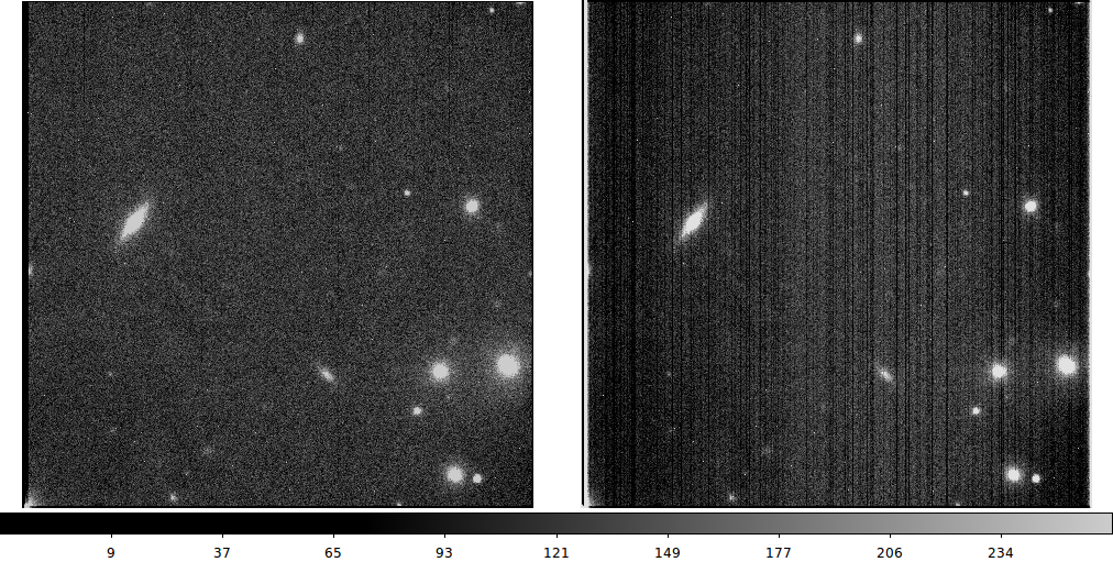
A typical example of the improvement we derive from a a simple bias
correction with the acm. A mean fixed bias pattern frame was computed
using nine bias images from the night of 20180115. The bias corrected
image in the left panel is from a 5 second acm image in the (Gunn) r
filter. The raw frame is shown in the right panel for comparison. It should be
noted that the mean sky signal in this corrected frame is 123.98 ± 0.03 adu.
For comparison, correcting a single bias frame (not used in the computing the
mean fixed bias pattern) yields a mean signal of 0.24 ± 0.02 adu.
|
The links in this paragraph are severly out of date. I retain them now only to
preserve some figures that remain of interest. I have some
early notes on bias abd dark frames with acm and some early
notes on processing multiple nights to investigate the bias and dark properties of
the acm data. I have also compiled
other notes that describe early studies of acm bias and dark properties.
The acm has a substantial fixed bias pattern (FBP) and the mean bias level
of the camera seems to float around the level of 1385 adu (± 6 adu).
# Building a master bias frame
% setenv date 20180206                    # optional
% acm_basic_list list.BIAS                # optional
% ds9_list_load list.BIAS                 # optional
% process_acm_bias list.BIAS 9 $date N
As you see, the only required step here is to run process_acm_bias, the script
that will stack (most or all) of the bias frame listed in the file list.BIAS. In
the first optional step I define a system variable named "date". I use this
as the identification string I feed to process_acm_bias (as arg3). The next
two optional lines allow me to view all of the images and summary information about
this. This sort of a last quality control check before assmbling the bias fame we'll
use to correct our acm images.
The images and files built isthis procedure are shown and explainsed below.
% ls
20180115T040325.2_acm_sci_BIAS_20180115.Explain		     20180115T040325.2_acm_sci_BIAS_20180115_margdist_col.table
20180115T040325.2_acm_sci_BIAS_20180115.fits		     20180115T040325.2_acm_sci_FBP_20180115.fits
20180115T040325.2_acm_sci_BIAS_20180115_margdist_col.parlab  list.BIAS

20180115T040325.2_acm_sci_BIAS_20180115.fits
   - The final master bias frame

20180115T040325.2_acm_sci_FBP_20180115.fits
   - The fixed bias pattern image (with a mean level of 0)

20180115T040325.2_acm_sci_BIAS_20180115_margdist_col.parlab,table
   - A table file of the column-averaged bias data from the stacked image

20180115T040325.2_acm_sci_BIAS_20180115.Explain
   - A summary file that contains information about the stacking
     process. One of the most useful parts of this file comes at the
     end where I list the images used inthe stack and those image NOT
     used in the stack. As we see below, it is usful to apply the final
     master bias frame to a single bias that was not used in building
     the master bias. This simple test will verfy that we properly remove
     fixed bias pattern and that our resulting produc has a mean level
     very close to zero.
Below I show two figures that demonstrate what we have done. The first (directly below)
show aspects of the master bias and it's application.
 |
|
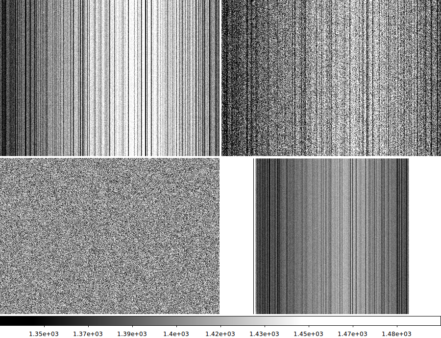
A section of the mean bias frame (a total of 21 acm bias frames) is shown in the
upper left. We see numerous vertical lines. In the upper-right is a single bias frame
of the same area (not included in the mean image stack). In the lower-left is the
same area of the single bias frame after subtracting the master mean bias. We see
a substantial improvement with regards to removing the fixed bias structure. Fianlly,
it the lower-right I show the full field image of the master bias frame to show the
large amount of bias structure in an acm image.
|
In our second figure I show how we can use the table file to build a plot that
shows the fixed bias pattern from our master stack using the
xyplotter_auto routine.
% cat 20180115T040325.2_acm_sci_BIAS_20180115_margdist_col.parlab
col   Column Number
mean  Mean signal value (adu)
sig   Standard devistion (adu)
me    Mean error about mean (adu)
Npix  Number of pixels

% xyplotter_auto 20180115T040325.2_acm_sci_BIAS_20180115_margdist_col col mean 1

# I use the matplotlib show() module I can adjust the plot as I see fit. I
  can also chhose to create a hard copy version of the plot, which I show below.
 |
|
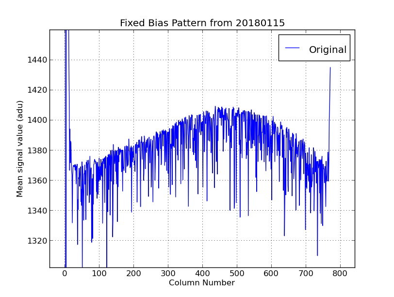
The fixed bias pattern computed with the process_acm_bias routine. Using the
matplotlib show() routine I have set the scale so that we can clearly see the
large scale properties of the acm fixed bias pattern. Despite the low resoltion
of this plot many of the bad columns in an acm bias are evident. The placement
and depth of these bad columns has remained fairly constant over the course of weeks.
Another major feature is the large-scale rise and drop in the bias signal across
the chip. The ammplitude of this feature is approximately 40 adu and hence is
extremely significant given that our average sky signals typically fall in the
range of a 50 to 300 adu. Furthermore, over a range of just 100 pixels (in the X
direction) the bias signal changes systematically by 10 adu or so (over much of
the image). Hence, without removing this source of systematic error, measurements
of profiles, sky surface brightness, or integrated magnitudes can be adversely affected.
|
Buildng a master darkrate frame.
This section need more detail.
# See example:   /home/sco/ACM_Red1/20180115/old_dark5
I made a single good darkrate image:  ./20180115/old_dark5/20180115T040719.0_acm_sci_DARKRATE_DARK5.fits

# Main tool to make the darkrate image
% process_acm_darkrate
Usage: process_acm_darkrate list.DARK5 5 20180116DARK5 MeanBias.fits Y
arg1 - list of input (bias) images (can be fullpath)
arg2 - number of images in each sub-stack (NSIZE)
arg3 - identification string (usually UT date of acm night)
arg4 - name of bias image to be subtracted
arg5 - run in verbose/debug mode (Y/N)

# To split exp times
% list_split_exptime ../list.OPEN ListEXP N
It seems best now to process darkrate images using darks that match
as closely as possible to exposure times of the sky images being reduced.
Note that I uusally find darkrates in range 0.3 adu/sec (good nights) to
2.0 adu/sec (bad nights).
Initial pipeline processing.
Once we havethe bias and dark images, we can process the acm images. Make a list of
the images to be processed by starting with my big list.OPEN from the run of
acm_list.
 % pwd
/home/sco/ACM_Red1/20180206/sky_5sec
% list_split_exptime ../list.OPEN ListEXP N
With the above command I created ListEXP.5sec (a list of my 444 5sec images).
In practice, I use environmental variables to define the paths to my bias and dark
images computed in the previous sections. Then I process the images listed in
ListEXP.5sec using acm_ccd_correct.
% echo $bias
/home/sco/ACM_Red1/20180115/Bias/20180115T040325.2_acm_sci_BIAS_20180115.fits
% echo $drate
/home/sco/ACM_Red1/20180115/dark5/20180115T040719.0_acm_sci_DARKRATE_DARK5.fits

% acm_ccd_correct ListEXP.5sec $bias $drate
*** To process 34 images tkaes about 10sec on scohome ****
*** To process 444 images tkaes about 4min on scohome ****
For convenience I move the processed (*_proc.fits) images to a subdirectory
and then review them with bigds9.
% ls -1 ./images/2018*proc.fits > list.proc
% bigds9 list.proc 16 16        # To see images in 4x4 tiled ds9 views
Install useful WCS solutions.
I have compiled some early rough, example-oriented, notes, but
the sequence of processing steps to derive WCS solutions continues to evolve with time. The
basic steps are fairly secure now, and I give a simple overview here. To see the specific
details using in this document, the reader shoudl refer to the End-to-End description
given above.
The basic steps for an acm image are as follows. We use the
wcsf_rough routine to graphically
identify a soirce of known Ra,Dec. This is done by simultaneously diplaying the acm image along
with a DSS image of (approximately) the same field. The scale and position angle values in a raw
acm image are usually approximately correct. IT is the sky zeropoint (i.e. the values of
CRVAL1,CRVAL2,CRPIX1,CRPIX2) that are usually off in the header by 5-20 arcseconds. Once these
values are reset, we have a WCS header that is already good enough to perform a lot of tasks.
Next, I visually confirm these rough fits and generate USNO-B1.0 astrometric catalogs for
each image using the wcsf_viscat routine. To create
catlogs of all sources detected above a user-specified sky threshold we next run the
wcsf_imgcat routine. In the last step we use the
wcsf_final routine to cross-match each image catalog
with the USNO sources and derive a new set of astrometric standards. A final, improved WCS
solution id computed and installed in the header of each image. The r.m.s scatter in both X,Y
for typical acm images vary between 0.2" to 0.8" and these values allow cross-matching with
PS1 data to allow photometric zeropoint derivation (see below).
Derive and install photometric ZP values.
Here I use the 14 wcs-calibrated images described in previous sections to
calibrate photometric zeropoints using PanSTARRS gri photometry. The
basic tool for this is photcal_fitslist,
which can use phtometry from both USNO-B1.0 and PanSTARRS to install photometric
zeropoint data into the headers of an inpu list of FITS images.
My top ZP reduction director is:
/home/sco/A_wcsf/ZP_may16

# In ./ZP_may16/S I make the image list
ls -1 /home/sco/A_wcsf/Run_apr17/local_red/WCS/20*fits > list.0

I create the ./local_red archive directory, then:
% photcal_fitslist ./S/list.0 ps1 N
If we reduce images using PanSTARRS photometry (via PS1) then we'll have to
do a second pass after the gri photometry (actually gri and transformed BVR
photometry) has been gathered.
After the images are calibrated when can make a summary table.
% cd ./local_red/ZP
% gethead *.fits FILTER PSYSNAME ZPSEC ZPERR NUMZP

F = FILTER name in the image header
S = standard photometric syystem transformed to
ZPSEC = ZP for a 1-sec exposure
err   = mean error of ZPSEC
N     = Number of points used to derive the calibration

Image Name                          F  S    ZPSEC    err    N
----------------------------------- -  -  -------- -------- --
20180206T022042.6_acm_sci_proc.fits B  B  -3.06280 0.020384 10
20180206T032156.5_acm_sci_proc.fits B  B  -3.30300 0.029670  4
20180206T035223.8_acm_sci_proc.fits B  B  -3.01700 0.023692  3
20180206T061218.4_acm_sci_proc.fits r` r  -2.56400 0.015604  4
20180206T070902.2_acm_sci_proc.fits r` r  -2.27517 0.023742  6
20180206T072507.6_acm_sci_proc.fits r` r  -2.63950 0.006500  2
20180206T083937.3_acm_sci_proc.fits r` r  -2.57000 0.025956  8
20180206T092518.0_acm_sci_proc.fits r` r  -2.50075 0.042880  4
20180206T100533.3_acm_sci_proc.fits r` r  -2.36000 0.028202  6
20180206T101258.1_acm_sci_proc.fits r` r  -2.22300 0.022627  8
20180206T102445.6_acm_sci_proc.fits r` r  -2.42300 0.027937  4
20180206T104913.4_acm_sci_proc.fits r` r  -2.95500 0.023624  8
20180206T105144.7_acm_sci_proc.fits r` r  -2.83483 0.020092  6
A working catalog and image header additions.
At the end of our reduction we want a working catalog that can be used for practical
purposes. By this I mean we desire some file(s) that contain astrometric positons (from
our WCS solutions) and calibarted photometry (from our zeropoint solution) in some standard
system. A couple simple goals for the work that motivated this document are:
- Cross-match observed acm phtometry with other catalogs to derive how
our calibratd aperture photometry compares to that in other catalogs.
- Derive photometrically calibrated sky surface brightness values from
acm images and study dependence on things like moon illumintaion and angle,
structure azimuth and tracker position, etc....
Below I list some of the basic tools I use for this step.
# Set and measure regions in the images
Usage: ds9_imstats a.fits Y
arg1 - FITS image name
arg2 - run in interactive mode (Y/N)

# Establish a table of Ra,Dec positions for eavery region (must have WCS)
Usage: midowcs ./S/20180206T022042.6_acm_sci_proc.fits N
arg1 - Name of FITS image (can be full path)
arg2 - run in debug mode (Y/N)

# Establish table and cdfp files with calibrated photometry
Usage: midophotcat.sh a.fits Y
arg1 - name of the LOCAL input FITS image file
arg2 - Run in debug mode
The basic catalog(s) made in this step can be used to address our two goals above.
The best wrapper tool for all of the aboveroutines is called "ds9_fitslist". It
allows you build ds9 region and mido information files for a list of images. If
the proper header information is installed, then a phtometric catalog is also prepared
in the form of a table file and a cdfp file. If desired, these data products for each
images are archived (in the CAT subdirectory). On subsequent runs of ds9_fitslist you
will be asked if you wish to start with these archived products. Here is a sample run:
% cd /home/sco/A_wcsf/ZP_may20

% cat ./S/list.test
/home/sco/A_wcsf/ZP_may20/local_red/ZP/20180206T020222.8_acm_sci_proc.fits
/home/sco/A_wcsf/ZP_may20/local_red/ZP/20180206T022042.6_acm_sci_proc.fits
/home/sco/A_wcsf/ZP_may20/local_red/ZP/20180206T032156.5_acm_sci_proc.fits

% ds9_fitslist ./S/list.test N
arg1 - Name of file with list of FITS images (can be full path)
arg2 - run in debug mode (Y/N)
The last step of the process here is to now take the results from
our ds9 runs, primarily the sky box flux measurements, and install them
and other useful values into the FITS header of each image. In particular,
we insert values aboit the moon (mmon illumination, monn separation angle) and
predicted model sky surface brightness into the header. I also run a
routine that computes the totaltracker offset from center and puts this into
the header. These setpas are all run by the routine acm_skysb_stats.
Here are some typical calls:
% acm_skysb_stats 20180403T042947.5_acm_sci_proc.fits Y N
% acm_skysb_stats 20180403T052406.0_acm_sci_proc.fits Y N
% acm_skysb_stats 20180403T053306.8_acm_sci_proc.fits Y N
As discussed in the End-toEnd doc presented above, I usually build a
script that runs acm_skysb_stats for all of the images I have processed in
a given night. A more efficient wrapper script that takes a list of input FITS
files may eventually be built.
Analysis
In the Appendix section below I have retained a set of notes that demonstrate an
early analysis of the acm phtometry results derived with this pipeline. The most
useful portion of this early work shows how I can compare the final acm photometry
with other sources (e.g. PS1 gri photometry). My use of the title "Analysis" for this
section is intentionally vague. The scope and golas of any analysis of an acm reduction
will surely change over time. Hence, I refer to a help document
that illustrates an anaysis of the header
information installed in the previous section. Basically, I use a variety of
Table tools to extract and order the header values for 90 images (my Bgr images from
five different nights) into a Table file. Using munging and table tools I have developed
I created the plots below. Note that the files and plots generated in this
work are arcived with this html document in $scohtm/Night_of_acm/work_analysis.
 |
|
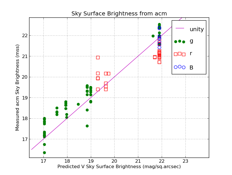
The sky surface brightness values from acm images taken in the B, g, and r filters.
These data were gathered from the FITS headers of 90 images and manipulated with
the table tools discussed in a document
with several examples. On the X axis above I plot the sky surface brightness
in the V-band predicted with a model developed from data obtained from a LaPalm
web site. The zeropoint of this relation (i.e. the V sky brightness in a moonless
sky) was taken from a study of the sky brightness at Mt. Graham by Taylor etal (2004,
PASP,116,762). This model uses the moon phase (illumination) and angular separtion from the
moon to predic the night sky brightness for each acm image. On the Y axis I plot
the g, r, abd B sky surface brightness estimates (in mag per sq.arcsec) derived from
acm images taken on 5 different nights. It should be noted that some of the g,r
data from the last night (20180403) may have been taken under partly cloudy conditions.
One thing to note is that the large clump of points around mu_V=21.9 are measurements
made under moonless conditions. It is peculiar that the r points taken under near full-moon
conditions lie above the unity line (fainter than the unity line) but below the unity line
in the case of moonless points. More g,r data taken on clear nights, under varying moon
conditions, is needed to resolve the source of this feature.
|
 |
|
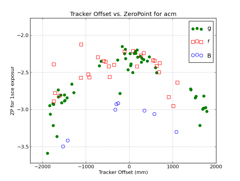
The photometric zeropoints for a 1 second exposure in g, r, and B as a
function of tracker offset. Here we see the clear trend in ZP with the
distance from tracker center for all 3 bands. The trackker offset, RSTRT, is
derived by combining the X_STRT and Y_STRT values in quadrature. The sign of
the X_STRT value is arbitrarily assigned to the value of RSTRT. Basically, we see
the role of pupil illumination variation as the HET tracker departs from the
track center. With more data from photometric nights we should be able to
derive or confirm a model of pupil illumination for the HET.
|
 |
|
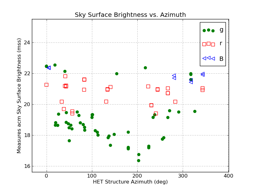
The sky surdace brightness in g, r, and B as a function of HET structure azimuth. We
have mixed the moon/moonless data sets, but it seems that the g data indicates the
sky is brightest in the south. However, most of these southern points were taken when
the moon was up (and in the south), and hence this is not surprising. What is needed
is a way to mask out the moonless nights (images with MILLUM=-999.0) and reconstruct
this plot. We need a tool to compute a table mask based on numerial values and this
is surrently being pursued.
|
A summary of the image material.
It is useful to summarize the location and purose of the image
directories used in this exercise. All of this work was done on scohome,
so I include the fullptah names for that machine. In the section below
I list the size of each major subdirectory. I start with an example of
how these sizes are found.
% du -sh /home/sco/HET_work/acm_nights/
21G	/home/sco/HET_work/acm_nights/

acm_nights
==========
21G	/home/sco/HET_work/acm_nights/
 - The raw acm images and the nightly RA logs are stored here. The sets are
   broken into the usual PAS data structures by UT night.

ACM_Red1
========
3.5G	/home/sco/ACM_Red1
 - Directories where I reduced and calibrated the acm images by UT night.
To get a list of all images that are fully ZP-calibrated:
% ls -1 /home/sco/ACM_Red1/2018????/SkyBoxes/local_red/CAT/*.fits >all.acm

SBsky_May2018_acm_reduced
=========================
207M	ACM_reduced_SBsky_May2018/
 - Collection of all calibrated acm image that I used to derive sky
   surface brightness values in g,r,B.
     -----------------------------------------------------------------------------------
     To collect these images in the SBsky_May2018_acm_reduced/acm   I used:
     % cp /home/sco/ACM_Red1/20180114/SkyBoxes/local_red/CAT/*.fits .     # 12 images
     % cp /home/sco/ACM_Red1/20180115/SkyBoxes/local_red/CAT/*.fits .     # 20 images
     % cp /home/sco/ACM_Red1/20180206/SkyBoxes/local_red/CAT/*.fits .     # 14 images
     % cp /home/sco/ACM_Red1/20180402/SkyBoxes/local_red/CAT/*.fits .     # 23 images
     % cp /home/sco/ACM_Red1/20180403/SkyBoxes/local_red/CAT/*.fits .     # 21 imags
     *** This is a collection of 90 images.
     -----------------------------------------------------------------------------------
We see the redection in total size with the sequence above.
Appendices: A variety of docs related to acm processing.
A host of early notes and links to useful documents have been
compiled in an Appendix Section.
Back to SCO code page