Here we discuss how to compute a radial profile. This can be used to describe a stellar PSF or the light distribution in a galaxy. Today the more frequently used approach is to fit the 2-D light distribution in such source using an analytical model and some optimization method. There is still a lot of utility in using the 1-D approach, and floowwing the "walk before you run" approach, I'll discuss some ways that I do that here.

1. A very simple graphical approach to profiles.
2. Some easy improvements.

In computing a 1-D (one dimensional) surface brightness profile for an image source, we are assuming the image has a symmetric radial light distribution. By this I mean contours computed at different have a circular of elliptical shape, and the center of each contour is the same. This is not always the case , as we'll see in our first exercice here with NGC3379, but is common enough for well-behaved images of stars and poorly resolved galaxy images. To begin, we'll look at some initial profile calculations I made using the simple graphic tool named ds9_profiles. The two main things we need for a profile is a center and an extent. The ds9_profiles tool allows us to use a ds9 regions marker to specify both on an image. We can also use markers to sky sky boxes and maybe some other useful properties in the image. Here are some notes from a "raw" run with ds9_profiles using a single B-band image of NGC3379 (named Rsco2042.fits). I include warts and all here to indicate some things might do to fix up the code and make it a little easier to use.

 
Usage: ds9_profiles dsi11.fits 120.0 LOCAL_SKY N 
Usage: ds9_profiles dsi11.fits 0.0 FIXED_SKY N 
arg1 - name of input FITS image file
arg2 - asemi_max (= 0.0 to use individual region sizes)
arg3 - sky (= FIXED_SKY, fits_image_name, LOCAL_SKY)
arg4 - file cleanup (Y/N)

% ds9_profiles Rsco2042.fits 0 FIXED_SKY Y
Fails, but I save:    p1.reg 
I can load it and use it in future runs.

Use same regions, but:
% ds9_profiles Rsco2042.fits 0.0 FIXED_SKY Y
So, we must specify using the region ellipse semi-major axis 
by saying R="0.0", not just R="0" 

The actual peak pixel position for N3379 is   X,Y = 1049,965
I fix this position, and a better ellipse, in:  p2.reg 
Yet, when I plot the growth curve, the title is 
telling me different:   X,Y=989,1037
Also, I get a shitty looking profile. What's up? 

Now I just turn off the clean-up request (arg4) and I see 
where that bogus center comes from: 
% cat profpars.out_explain
# Output columns from profpars (using midodata.2)
Col01 = X center, pixels (from centroid)
Col02 = Y center, pixels (from centroid)
Col05 = semi-major axis length in pixels  
Col06 = b/a axis ratio
Col07 = position angle (degrees) of major axis 
Col08 = local background 
Col08 = mean background (signal per pixel)
Col08 = mean error of background (signal per pixel)
% cat profpars.out
     989.300     1037.690      137.412  0.87734  -64.277     230.8790     222.2015       6.1598
                                                                        sky is okay
So, the local sky look reasonable, but the X,Y are not what I 
thought I was setting via the regions file. What is going on? 

The answer seems to be:
I display and set regions, but then I use profpars.sh to get the 
ACTUAL profile parameters (which are always in a local file that 
is named "profpars.out"). For my one ellipse here I get:
% cat profpars.out_explain
# Output columns from profpars (using midodata.2)
Col01 = X center, pixels (from centroid)
Col02 = Y center, pixels (from centroid)
Col05 = semi-major axis length in pixels  
Col06 = b/a axis ratio
Col07 = position angle (degrees) of major axis 
Col08 = local background 
Col08 = mean background (signal per pixel)
Col08 = mean error of background (signal per pixel)
% cat profpars.out        
     989.300     1037.690      137.412  0.87734  -64.277     230.8790     222.2015       6.1598

**** And here is my probable answer: the centroid center, 
     which involves the WHOLE ellipse is not on the galaxy 
     peak (nucleus). What is the best (i.e. clearest to the 
     user) way to fix the profile center on the PEAK? 

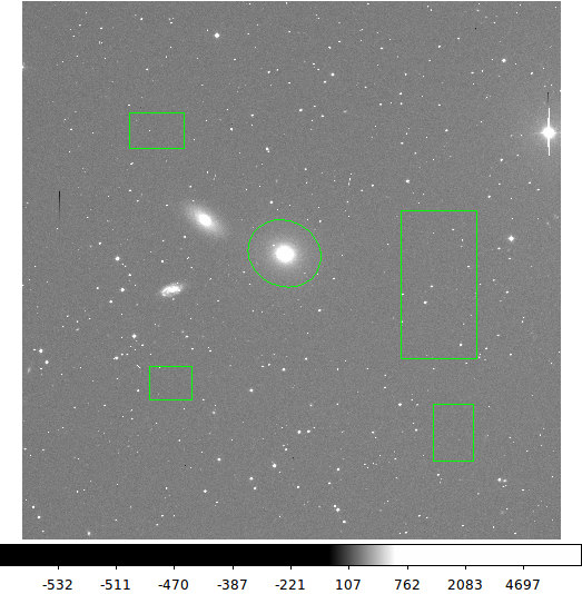
The ds9 view of Rsco2042.fits, our test image of NGC3379. With ds9_profiles we have displayed the image and marked NGC3379 with an ellipse marker. We have also specified 4 sky boxes that we'll use (via the MIDO routine inside ds9_profiles) to compute a global mean background value for the image.

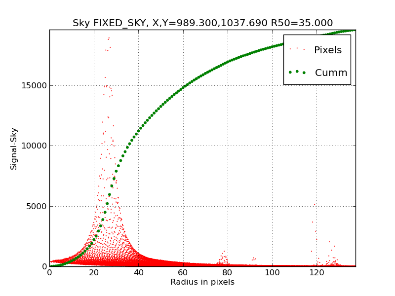Here is the profile we derive from our first run of ds9_profiles using the regions specified in the figure above. The command I used was: % ds9_profiles Rsco2042.fits 0.0 FIXED_SKY Y We've used the global mean sky value for the image (FIXED_SKY) as opposed to the local value around our ellipse regin (LOCAL_SKY). As we see, the resulting profile is not very pleasing. The large "bump" of excess light in the radius range 20pix to 40 pix is caused by the fact that our centroid center (X,Y=989,1038) is really quite far from the real position of the nuclues (X,Y = 1049,965). So, our first question becomes: how can we compose a practical way of "telling" ds9_profiles that we want to use the nucleus position instead of the centroid center. A broader question might be: how often does such a thing happen? The light distribution of NGC3379 is extremely smooth and symmetric compared to most galaxies. Maybe this sort of thing will be quite common. Notice alos the there are a few more "bumps" of light in the outer extent of the profile. These are bright stars in the image that have nothing to do with the light from NGC3379. How should we eliminate the effect of these stars? See below for the full explanation, but the biggest error in making the above profile had to do with some bad header cards and causing a misplaced radius model in the rad.fits image made by the ellradius.sh code.

1. I could make the code recognize a default regions file from the start? This would speed things up for the user, and let them more easily build more and more complicated region files.
2. I can just give the user the option of hand editing the profpars.out file. Just a low-tech for approach for now.

Based on the last considerations above, I have decided to quickly review the guts of ds9_profile (as it stands now) and discuss some easy ways to attain versatility and clarity during use. Here is what happens when we execute ds9_profiles:

1. The ccdsize script is used to derive the size of the input image.
2. If a "midodata.2" file is NOT present, then we open a ds9 gui with ds9_open (bash), display the input image with imlook (bash), set region markers with ds9_id (bash), then run profpars.sh (OTW) to compile paramters for regions we'll derive profiles for (currently ellipse and circle markers).
3. For each entry in the file "profpars.out" (from profpars.sh) we build a radius map with ellradius.sh (OTW), collect the profile points with profile_pnts.sh (OTW), and compute a growth curve with profile_gcurve.sh (OTW).
4. Lastly, for each profile, we construct a plot with profile_plot_01.py (python) and display it interactively.

As often happens, I had some "bad" header cards in my test image: Rsco2042.fits. At least one of the cards was throwing off my coordinates, and some of the bad features of my profile were due to my improper placement of the radius image model. I used the routine remove_fits_kwords to fix this up. Briefly, here is what I did:

 
% cat bad.keys
CCDSEC  
ORIGSEC 
PROGRAM 
DETECTOR
SSI     
PREFLASH
GAIN    
RDNOISE
CAMTEMP 
DEWTEMP
CCDSUM  

% remove_fits_kwords Rsco2042.fits bad.keys

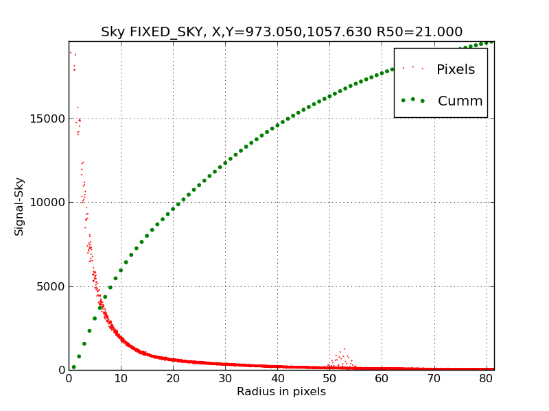
Now this is more like it! Here we see the ds9_profiles result after I have used the remove_fits_kwords routine to delete a bunch of bullshit FITS header cards that were causing differences between the image and physical coordinate systems. This was causing the radius image model to be placed incorrectly. Hence, my profile and growth curve estimates were completely messed up. However, the changes I have added to ds9_profiles remain valid and useful. Note that we would still see some "splitting" of the profile points in the inner region we used the centroid center at X,Y=974.1,1056.8 (see figure directly below). In this case, I altered the ellipse region center based on the peak value and edited in the nucleus position of X,Y=973.4,1057.2, and we see a much smoother profile.

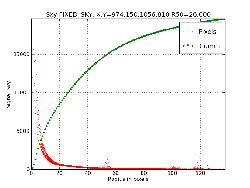
Here we have used the LOCAL_SKY and the ellipse region paramteres defined by the large outer ellipse. The centroid center at X,Y=974.1,1056.8 creates an "offset nucleus" situation in the inner profile. A graphical means of assigning a "user-specified" center is our next goal in our set of simple additions to ds9_profiles.

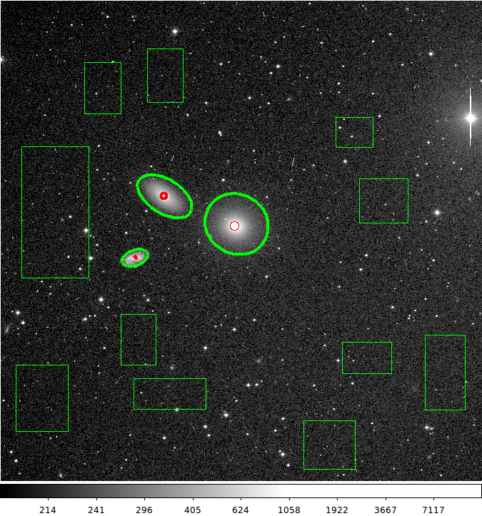Here we have used the (new as of Nov2015) ability of ds9_profiles to specify the center of an ellipse profile aperture. The small (red) ellipse markers are used to isolate the (X,Y) center we want for each elliptical profile, The colors do not have to be red, but I made them that way here to illustrate more clearly what is happening. This image and the markers seen above can be reporduced withthe TDATA exercise in: $tdata/T_runs/profiles/ex1_n3379