Image Photometry(Begun: April 2015)
Here we discuss how to use some of the tools in my scocode table to measure
some simple properties.I have a lot of specialized tools and
scripts, but most of the time we want an easy, direct way to:
- Open a ds9 window and show a well-scaled image.
- Mark objects on the image using different apertures.
- Obtain measurements (i.e. magnitudes, positions, profiles, etc..) of
the objects.
The exercises described below allow us to accomplish these tasks.
The exercises are meant to roughly build on one another. We can first
use a few simple aperture measurements (Exercise 0) to get a rough idea
of the properties of our image: background level, peak flux values,
photometric zeropoint, etc... Next, we may want to characterize the
size of the stellar seeing disk using a radial surface brightness
profile (Exercise 1).
- Exercise 0: View and Measure an Image.
- Exercise 1: Compute and Plot a Radial Profile.
Exercise 0: View and Measure an Image.
In the early sections here we'll go to the Test_Data (cd $tdata)
location and test a simple measurement procedure using an image near
the cluster NGC869.
- Get the image.
- View the image.
- Specify and measure image regions.
- Derive a photometric zeropoint.
Get the image.
We get started by getting to our working directory and copying over the image
file (n869.fits) that we'll view and measure.
- Use the "got" alias to go to the Test Data
% cd T_runs/Image_Photometry/ex0
% S/GRAB == To get the image n869.fits
The GRAB script is just a simple routine for pulling over our test image
(which is n869.fits in this example).
View the image.
Next we want to open a ds9 window and display the image. We'd like to have the
image grey-scale level set well enough from the start that we'll see something
immediately. The routines "ds9_open" and "imlook" will do this nicely.
Usage: ds9_open 800 800
arg1 - X size (800)
arg2 - Y size (800)

% ds9_open 800 800

Usage: imlook a.fits 15.0
arg1 - name of FITS file to be viewed
arg2 - Sigma-level for high end grey level (z2)

% imlook n869.fits 20
User z2 = 24.740
The first command opened a ds9 window of size 800x800 (a good size for mcs), and the
second displays the image (n869.fits). One advantage of using "imlook" (IMage LOOK)
is that it runs the cih.sh (Compute Image Histogram) and derives an estamate of the
image background. Using this "sky" level it then estimates an upper level (z2) for
setting the ds9 grey-scale. In this case, we requested that the top grey-scale level
(z2) be set at 20-sigma, where sigma is the standard deviation of the sky level. For most
astronomical images, this will allow us to see stars and some features in extended
sources (like galaxies). If you want to see fainter (lower surface brightness) features,
then use a lower value for argument 2 (like 5).
Specify and measure image regions.
The previous steps have been rather mundane and easily reproduced manually. However, in
this section we use a variety of codes and scripts to perform some highly generic and
useful steps. We use the "ds9_id" script to mark regions and measure them. In this case
I use the term region (as it is called in ds9) to denote an aperture. I want to draw a
box, circle, or ellipse, and then compute the sky-subtracted total flux within that
region. Here's how to do it:
Usage: ds9_id a.fits Y Y
arg1 - name of input FITS image file
arg2 - Y/N for column explanation table
arg3 - Y/N for automatic JPEG generation
% ds9_id n869.fits Y Y
Just a few quick words about the Y/N queries we had to include above. For a lot of uses,
we want to generate a table of measured parameters and view them on the monitor. In most
cases like this, we want to also view some explanation of what the columns are. This is what
we get if we we answer "Y" for argument 2 (i.e. a listing of column explanations followed by
the data table). However, we may want to direct the "ds9_id" output to another file and use
it in a script somewhere downstream. In order to more easily acces this file, we may want to
skip the explanation lines (an hence we would answer "N" for arg2). As for the last argument,
if we answer "Y" on arg3 we'll generate an image of final ds9 view. It may be useful to
preserve a view of the image markers. Currently, the name of this image will is fixed to be
"a.jpeg" and hence it will be overwritten in subsequent runs, so be sure to rename the jpeg
file if you want to preserve it.
After executing the ds9_id command above, I marked some regions and hit a RETURN. At that point
the ds9_id script stored the region properties to a local information file (named n869.info),
computed region properties, and generated a table of values on the screen. It also generated
the jpeg file that I display below under the generated table of values:
# Contents of:  midodata.2
Col01 = X pixels (aperture X center)
Col02 = Y pixels (aperture Y center)
Col03 = X center, pixels (intensity weighted centroid)
Col04 = Y center, pixels (intensity weighted centroid)
Col05 = magnitude (assuming zp=30)
Col06 = Average value per pixel in aperture
Col07 = Average value per pixel in annulus
Col08 = number of pixels in aperture
Col09 = Peak pixel value (image ADU)
Col10 = marker code (1=circle,2=box,3=ellipse)

   495.17    581.68    493.38    584.50  21.792     2.017     0.942     1785.0      25.00   1
   494.09    586.22    492.84    585.24  21.775     1.765     0.935     2350.0      25.00   2
   495.17    581.68    493.06    583.86  21.733     1.314     0.917     5104.0      25.00   3
   336.26    816.38    329.67    815.99  26.932     0.871     0.870    16044.0     239.00   2
   805.76    393.80    803.22    391.38 -99.000     0.594     0.618    12782.0      61.00   2
   640.03    239.63    628.94    236.34  19.995     2.662     1.011     6083.0     110.00   2
Some words on mido:
Inside the ds9_id script is
a call to the work-horse routine mido,sh (MIDO = Measure Image Display Objects). For our
photometry we are usually concerned with the mido measures in box, circle and ellipse
regions. It should be noted that for each region and "annulus" with same shape as the
input region is used to derive the local background (for subtraction). The size of this
annulua is currently set in the subroutine set_mido_pars in mido.f, where I define a fractional
aperture area compared to the primary aperture. The inner annulus has a size which gives
an area that is 1.2 times the primary aperture area, and the outer annulus will give
2.5 times the primary aperture area. It may be necessary at some stage to make these
values adjustable.
Finally, the ds9_id run will produce a few other useful files:
id.objects:
A listing with the region parameters for every object identified. The
basic parameters are ouline in the file header:
# Parameter Data Structures
# circle   == x,y,r
# box      == x1,x2,y1,y2
# line     == x1,y1,x2,y2
# text     == x,y
# ellipse  == xe,ye,aiso,biso,pa
A table follows which describes every target:
# data
circle     green          1076.260      592.462      235.513        0.000        0.000
box        green           175.524      444.464      812.310     1098.326        0.000
box        green           113.626      427.389      176.246      295.774        0.000
box        green          1590.661     1878.811       63.120      276.564        0.000
midodata.1 and midodata.1_explain
% cat midodata.1_explain
Col01 = original marker number (integer i10)
Col02 = marker type (1x,a10)
Col03 = marker color (1x,a10)
 |
|
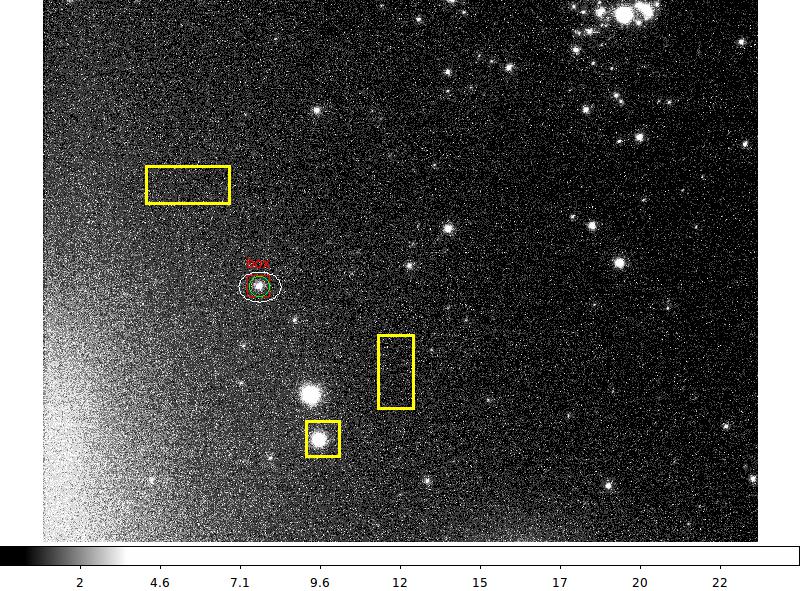
The ds9 image generated above using n689.fits. Notice that I have
set 6 ds9 markers (with different colors, line widths, and
one has a text string attached). The color information and such is
NOT displayed in the table, but it is preserved in the associated
information file (n689.info). Numerical information for each each
region is displayed in the Table shown above this figure. In particualar,
notice that the first three regions surround the same star (at roughly
X,Y=495,583). We see that regardless of the type of aperture we have
used (circle, box, or ellipse) the (sky-corrected) integrated magnitude
(Column 4 in our table) for these regions are closely the same values
(as they should be for a simple source such as this).
|
Notice in the table above that the first three regions above,
although different in type (shape) give closely the same
sky-subtracted total flux. Because these three regions
encase the same object, they all have the same peak pixel
values of Fpeak=25.0 (this is a simple way to estimate peak
flux, but it can come in handy at the telescope when trying to
derive an integration time that avoids saturation). Also, note that
the 3 yellow boxes show some interesting properties. The second box
has an average in the "annulus" value (i.e. the background value) that is
larger (per pixel) than the flux measured inside the box aperture. This
would mean that the integrated flux in the box, after sky subtraction, would
have a negative value. This can not be used to compute a magnitude, and
so the value of -99.0 is displayed in column 5 of the table.
Derive a photometric zeropoint.
The goal here is to be able to estimate the magnitude of star (or any source) in
our image. I show a few useful commands that tell me some properties of our image
(n869.fits) and get us started. Note that the image n869.fits is assumed to have a
proper WCS (World Coordinate System) installed in the image header.
% ccdsize n869.fits
1624 1234

Hence, the central pixel is Xc,Yc = 812,617, and we derive can the RA,DEC of the center
of our WCS-calibrated image with:
% xy2sky n869.fits 812,617
02:17:32.005 +57:05:09.45 J2000  812.000  617.000

To get a cdfp catalog and regions files for stars and gals:
% usno_look 02:17:32.005 +57:05:09.45 1.0 18.0
At this stage we'll have created a DSS image (dss.fits) and some catalogs (usno_all.cdfp,
usno_targs.cdfp) of sources in the field of that image. The usno_look script will display in
a ds9 window the sources overplotted on the image. An example is shown below where I have
added one feature manually to illustrate a feature of calling usno_look: the small green
vector shows that our field has a "radius" of 1 ARCMINUTE, as requested by our value of
argument 3 on the command line above.
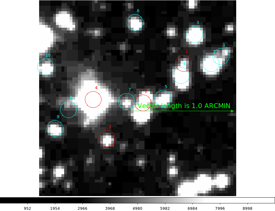 |
A simple run of usno_look gives us (mostly) the image
we see above. I say "mostly" since I have manually
inserted the green vector marker to show that the
extent of the DSS view is 1 arcmintute from the image
center to the right-hand (WEST) edge of the image. The
command I use to obtain this view was:
usno_look 02:17:32.005 +57:05:09.45 1.0 18.0
The last argument (18.0) is the limit (in V magnitude) for
objects that I want to gather from the USNO catalog. In the
figure above, objects selected as STARS are plotted
in RED, and objects selected as GALAXIES (or really as
non-stellar) are plotted in CYAN. The number associated with each
source is just a running integer.
|
Actually, the figure above is only partially useful. The "Names"
attached to the targets that are marked are simply the line
numbers of the sources in each region file. A better approach (which
has now been implemented in Apr2015) is to use the line number in the
original cdfp catalog file used to generate the region files (in
this case usno_look generates a catalog called "usno_targs.cdfp"). An
even more useful approach is to label the targets of interest using
a quantity. For instance, in the example below I show the targets
labeled with the V magnitude of each identified source. This will give
an easy way to compute a photometric zeropoint by identifying well-isolated
stars with magnitudes.
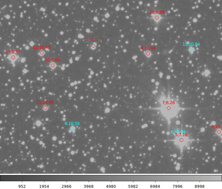 |
In the directory where I was to run usno_look I placed
a file named "extra.quantity" that contained the name of the
quantity I wanted to plot (the names are specified on the
first line of each cdfp file). In this case the name of
the quantity is "V" (i.e. the V magnitude generated for each USNO source).
usno_look 02:17:32.005 +57:05:09.45 10.0 11.0
After executing the above command, my image appears and I am
asked if I want to save a jpeg image. I can adjust the ds9
image any way I wish (as I did here by zooming to a better
view) before saving the jpeg. Note above that now the targets
are labeled not only with line number "names", but also the
tabulated V magnitude (after the semicolon) for each labeled source.
|
Hence, we could now use the jpeg image just produced and then
use the commands above (ds9_open, imlook, and ds9_id) to
measure instrumental magnitudes for appropriate stars (i.e.
bright, isolated, etc...) that have labeled V magnitudes.
After running ds9_id I could quickly build this table:
   X         Y      mag30       Fsky   Fpeak       V      Tsec  Fsat
  493.75    582.97   21.934     1.035   25.00      8.88   30.0  255.0
  574.92    504.20   23.297     0.927    9.00     10.04   30.0  255.0
  920.28    713.91   21.716     0.541   27.00      8.57   30.0  255.0
  629.56    233.75   20.026     1.061  110.00      7.16   30.0  255.0
  605.69    333.81   19.118     1.156  235.00      6.26   30.0  255.0
 1307.59    635.76   21.162     0.327   44.00      8.26   30.0  255.0
 1246.48    717.66   21.893     0.301   27.00      8.69   30.0  255.0

Using the File > "Display Header" option in ds9 I found that the integration
time for this CAT image was 30 seconds:
EXPTIME =                30000   (milliseconds)
With the table above, I can build a script to run the zpmido script:
% cat RUN_1
#!/bin/bash
#
zpmido.sh 21.934 1.035  25.00  8.88   30.0  255.0
zpmido.sh 23.297 0.927   9.00 10.04   30.0  255.0
zpmido.sh 21.716 0.541  27.00  8.57   30.0  255.0
zpmido.sh 20.026 1.061 110.00  7.16   30.0  255.0
zpmido.sh 19.118 1.156 235.00  6.26   30.0  255.0
zpmido.sh 21.162 0.327  44.00  8.26   30.0  255.0
zpmido.sh 21.893 0.301  27.00  8.69   30.0  255.0

% RUN_1
-16.747     8.636   319.216
-16.950     8.615   947.603
-16.839     8.434   289.127
-16.559     8.560    70.223
-16.551     8.490    32.714
-16.595     8.668   175.165
-16.896     8.563   286.528

% cat zpmido.explain

Output values:  z, zpeak, Tsat
z = instrumental zeropoint  =   -16.896
Tsat = time (in seconds) to saturation =     286.5

 mag_S = z + 30 - 2.5log(Fss) + 2.5log(T)

where,
mag_S = magnitude in standard system
Fss   = sky subtract total flux
T     = integration time in seconds
Fsat  = saturation level =     255.0

Also useful:
Tsat = 10.0^expon
where,
expon = 0.4 * {mag_S - zpeak + 2.5*log(Fsat)}
Tsat  = time in second to reach saturation
The zpmido.explain file is produced everytime the zpmido script is run.
It gives you the working equation to be used in computing a standard
magnitude using the time and zp value for an image. To get a mean
zeropoint, I would just direct the zpmido output to a file, and then
process that file with calstats.py:
% cat zp.dat
-16.747
-16.950
-16.839
-16.559
-16.551
-16.595
-16.896

% calstats.py zp.dat
-16.734 0.155 -16.950 -16.551 7
(mean,std,min,max,Npnts)

From the above I could then say:
 = -16.734 -+0.06

Hence, I could convert any magitude for a CAT image with:

   V = -16.734 + m30 + 2.5logT

where our standard magnitude fed to zpmido is in the V systsem
and the integration time, T, is in units of seconds.
In the same manner, I compute a mean zpeak in order to be able
to estimate the integration time (Tsat) needed to saturate a star
of a given magnitude (V):
% cat zpeak.dat
8.636
8.615
8.434
8.560
8.490
8.668
8.563

% calstats.py zpeak.dat
8.567 0.076 8.434 8.668 7
(mean,std,min,max,Npnts)

Hence, I derive:     = 8.567 -+0.03
Exercise 1: Compute and Plot a Radial Profile.
In the above (Exercise 0) section we made rather simple (global)
measures in apertures. We often want a more detailed description of
the light distribution in an aperture such as that provided with
a radial brightness profile. With a profile we can derive some
seeing width like a gaussian sigma, a full-width half max (fwhm), or
an encircled energy within the half-light radius (EE50). Information
about what constitutes an unresolved soure (i.e. a star) will be
crucial to analyzing unresolved sources (galaxies). Even more
complicated approaches can be used to describe differences in the
1-D profiles of galaxy light profiles.
I present a general discussion of
how I extract and display profiles here.
Back to SCO CODES page