This describes a second example of plotting multiple data sets with the xyplotter_auto and xyplotter routines. I had a collection of table/parlab files that gave pointing errors measured with the HET acm on different dates. These data are in the html docs directory:

 

% cd $scohtm/scocodes/xyplotter_auto/example3

% ls
20180401.parlab  20180402.parlab  20180403.parlab  20180404.parlab  20180405.parlab  20180406.parlab  Axes.1  S/
20180401.table	 20180402.table   20180403.table   20180404.table   20180405.table   20180406.table   List.1

% cat 20180402.parlab
dX   (Xbib-Xp) in arcseconds 
dY   (Ybib-Yp) in arcseconds

% head -6 20180402.table
# Col01: Xbib-X 
# Col02: Ybib-Y
# data
   8.525    9.240 
   1.270    8.794 
 -20.789   14.922 

Build the first plot 
% xyplotter_auto 20180401 dX dY  1

# Then I edit the List.1 file to add my other plots 
% cat List.1
% cat List.1
20180401.table 1 2 0 0   pointopen    r v 30    20180401 
20180402.table 1 2 0 0   pointopen    r ^ 30    20180402 
20180403.table 1 2 0 0   pointopen    r o 30    20180403 
20180404.table 1 2 0 0   pointopen    r s 30    20180404 
20180405.table 1 2 0 0   point        b o 30    20180405 
20180406.table 1 2 0 0   point        g o 30    20180406 

# I also editted the Axes.1 file a little
% cat Axes.1
Point Test Data
  -40 40  (Xbib-Xp) in arcseconds 
  -40 +40 (Ybib-Yp) in arcseconds 

Build the new plot
% xyplotter List.1 Axes.1

 

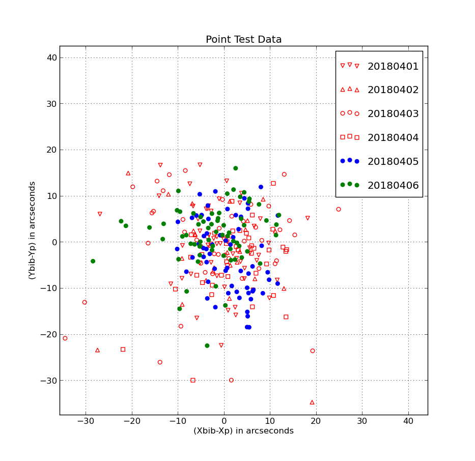I have combine 6 sets of HET pointing data (covering 6 nights) with: % xyplotter_auto 20180401 col mean 1 % xyplotter List.1 Axes.1 % cat List.1 20180401.table 1 2 0 0 pointopen r v 30 20180401 20180402.table 1 2 0 0 pointopen r ^ 30 20180402 20180403.table 1 2 0 0 pointopen r o 30 20180403 20180404.table 1 2 0 0 pointopen r s 30 20180404 20180405.table 1 2 0 0 point b o 30 20180405 20180406.table 1 2 0 0 point g o 30 20180406 / The six data sets are fairly clear in the plot, but you could easily alter the List.1 file to change the clarity of any given set.