 |
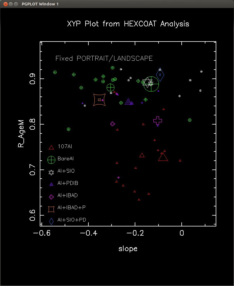
A plot from XYP. This is from a screen-grab
of the XWINDOW image that XYP gave while
running the code. I save the image as "ee.png" and to make a jpeg
from my I used the following command:
convert ee.png example_01_window.jpeg |
XYP is a general-purpose XY plotting package. It is designed to allow the user to inspect data plots interactively. Hard-copy versions of the final files are then generated.
|
A plot from XYP. This is from a screen-grab
of the XWINDOW image that XYP gave while
running the code. I save the image as "ee.png" and to make a jpeg
from my I used the following command:
convert ee.png example_01_window.jpeg |
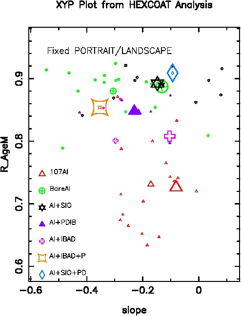 |
A plot from XYP. This is from the hardcopy
PostScript file made in PORTRAIT mode. To make a jpeg from my
PORTRAIT plot I used the following command:
convert xyplot_port.ps -resize 100% example_01_postscript_PORTRAIT.jpeg |
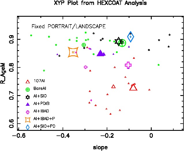 |
A plot from XYP. This is from the hardcopy
PostScript file made in LANDSCAPE mode.
To make a jpeg from my LANDSCAPE plot I used the following command:
convert xyplot_land.ps -rotate 90 -resize 100% example_01_postscript_LANDSCAPE.jpeg |
An ASCII file of any name (fin*120) is read to get the X,Y data. At this time no header lines are allowed. The file can contain multiple columns. In interactive mode, the user is queried for the names of parameters to be plotted, and the labels to placed on each axis.
Here is a sample input file called "t.1"
-----------------------------------------------------------------
# data
3
X
Y
Z
  680.040   6670.794   1.0
  769.710   7281.222   1.0
  824.070   7626.152   1.0
  841.200   7730.892   1.0
  889.080   8013.635   1.0
-----------------------------------------------------------------

*** Just answer questions in interactive mode, and you can
    plot X,Y values. The points will default to red dots.

How do we get different point types, colors, and sizes?
ANSW: Your input table must have columns with the recognized names
      "point_color", "point_type", "point_size".

The values of these point parameters are strings (NOT the PGPLOT
integer values, the routines in ipgtools called pgcfill and
pgtfill interpret the point color and type respectively.

Here are the recognized POINT TYPES:
      pgtypes( 1) = "point               "
      pgtypes( 2) = "cross               "
      pgtypes( 3) = "asterisk            "
      pgtypes( 4) = "circle              "
      pgtypes( 5) = "tilted-cross        "
      pgtypes( 6) = "open-square         "
      pgtypes( 7) = "open-triangle       "
      pgtypes( 8) = "circle+cross        "
      pgtypes( 9) = "circle+dot          "
      pgtypes(10) = "open-curvy-box      "
      pgtypes(11) = "open-diamond        "
      pgtypes(12) = "open-star           "
      pgtypes(13) = "solid-triangle      "
      pgtypes(14) = "stellated-cross     "
      pgtypes(15) = "star-david          "
      pgtypes(16) = "solid-box           "
      pgtypes(17) = "solid-circle        "
      pgtypes(18) = "solid-star          "
      pgtypes(19) = "big-open-box        "
      pgtypes(20) = "small-open-box      "
      pgtypes(21) = "circle-1            "
      pgtypes(22) = "circle-2            "
      pgtypes(23) = "circle-3            "
      pgtypes(24) = "circle-4            "
      pgtypes(25) = "circle-5            "
      pgtypes(26) = "circle-6            "
      pgtypes(27) = "circle-7            "
      pgtypes(28) = "arrow-left          "
      pgtypes(29) = "arrow-right         "
      pgtypes(30) = "arrow-up            "

Here are the recognized POINT COLORS:
      pgcol( 1) = "black-white           "
      pgcol( 2) = "red                   "
      pgcol( 3) = "green                 "
      pgcol( 4) = "blue                  "
      pgcol( 5) = "aqua                  "
      pgcol( 6) = "magenta               "
      pgcol( 7) = "yellow                "
      pgcol( 8) = "orange                "
      pgcol( 9) = "pea-green             "
      pgcol(10) = "light-green           "
      pgcol(11) = "light-blue            "
      pgcol(12) = "purple                "
      pgcol(13) = "light-red             "

The POINT SIZE is read as the usual floating point PGPLOT
expand factor.

Here is a sample input file called "t.2"
-----------------------------------------------------------------
# data
6           (# number of table columns)
X
Y
Z
point_color
point_type
point_size
  680.040   6670.794   1.0  green    cross        1.2
  769.710   7281.222   1.0  blue     circle       1.2
  824.070   7626.152   1.0  yellow   solid-star   1.2
  841.200   7730.892   1.0  red      solid-star   1.2
  889.080   8013.635   1.0  red      circle       1.2
-----------------------------------------------------------------
At this point, we could use a simple ASCII file to make the majority of the plots I would normally need to make. One test sample that will reside with the XYP source code and my Test_Data_for_Codes/T_runs examples is show below where I have simply run XYP in default mode. Below I show the portait mode PostScript file that is made (xyplot_port.ps).
 |
A plot from XYP using the test data in S/xyp/T/S8_skyplot. The plot has been reduced to 75% of it's original size. |
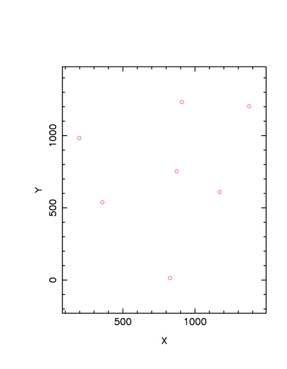
To control the page size and the dimensions of the plot axes, we can construct a local file called "xyp_plot.SIZE" that contains the values desired. All dimensions (i.e. all values except aspect) are specified in units of inches. To specify the virtual plot limits use a local file called "force.limits" contained the desired bounds (x1,x2,y1,y2).
Here is an example of "xyp_plot.SIZE":
9.0 1.0                 (xpsize,aspect)
1.00 7.75  1.25 8.00    (xleft,xright,ybot,ytop)

Here is an example of "force.limits":
-1.0 1.0 -1.0 1.0
In the shown below I have again used the S8_skyplot data to plot 7 X,Y positions. In this case I used the local xyp_plot.SIZE and force.limits files discussed in the figure caption. The important thing is that I made a plot whose bounds were 4 inhes in X and 3 inches in Y.
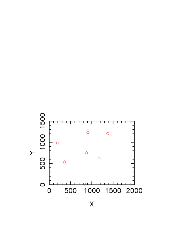 |
A plot from XYP using the test data in Files I used: % cat xyp_plot.SIZE 9.0 1.0 (xpsize,aspect) 2.00 6.00 2.00 5.00 (xleft,xright,ybot,ytop) % cat force.limits 0.0 2000.0 0.0 1500.0 The correct axis sizes and plot ranges were produced with this setup. Hence, it is fairly easy to make plots, like plots of sky coordinates, to match a desired physical scale. |
To control the page size and the dimensions of the plot axes, A local file called "xyp.input' can be made that specifies a lot of the stuff needed for the XYP run. Local files AXIS.LIMITS and xyp_plot.SIZE can be used to set plot bounds and sizes.
*** N.B.
The strings that go into AXIS.LIMITS are the actual axis
labels (not the variable names)!!!
i.e. we use "Y (HET mirror system)", not "Yhet"

For a nice plot of HET tracks, for example:

xyp.input:
track_BSC5-4388.xypdat
Xhet
Yhet
X (HET mirror system)
Y (HET mirror system)
HET Track for BSC5-4388

AXIS.LIMITS:
Xhet
-1.0 1.0
Yhet
-1.0 1.0

xyp_plot.SIZE:
9.0 1.0                 (xpsize,aspect)
1.00 7.75  1.25 8.00    (xleft,xright,ybot,ytop)

-------------------
So, by typing XYP in the dir with these files (and the data
file called track_BSC5-4388.xypdat, made by HAT) we get an
immediate plot of a track.

An example of this is shown in: S4_het_tracks/

Finally, in S4_het_tracks/xyp_script I show an example
of a little script *that can be installed in .../bin) to
do everything automatically:
(pt = Plot Track)

pt 4388

Here is a copy of the current pt:
----------------------------------------------------------------------
#!/bin/sh
#
# usage:
# pt ####
#
echo "   "
echo "usage:  pt ####                        "
echo "where #### is the Yale BSC star number "
echo "   "
echo 'track_BSC5-'$1'.xypdat'  > xyp.input
echo 'Xhet                  ' >> xyp.input
echo 'Yhet                  ' >> xyp.input
echo 'X (HET mirror system) ' >> xyp.input
echo 'Y (HET mirror system) ' >> xyp.input
echo 'HET Track for BSC5-'$1  >> xyp.input
#
echo 'X (HET mirror system) '  > AXIS.LIMITS
echo '-1.2 1.2' >> AXIS.LIMITS
echo 'Y (HET mirror system) ' >> AXIS.LIMITS
echo '-1.2 1.2' >> AXIS.LIMITS
#
echo '9.0 1.0                 (xpsize,aspect)          ' > xyp_plot.SIZE
echo '1.00 7.75  1.25 8.00    (xleft,xright,ybot,ytop) ' >> xyp_plot.SIZE
#
date > clean.skip
echo '   '
XYP
#
mv xyplot.ps track_plot_YSBC$1.ps
#
# To display
#vps track_plot_YSBC$1.ps
echo 'To print:'
echo 'lpr -Phetsneed track_plot_YSBC'$1'.ps'
echo 'lpr -Psneed track_plot_YSBC'$1'.ps'
echo 'lpr -Praprint track_plot_YSBC'$1'.ps'
----------------------------------------------------------------------

***** A full blown HexBurst example.
* See files in src/xyp/T/S4_het_tracks/S_with_hat:
  - run HAT with skytools option to make the files:
    track_BSC5-4335.xypdat
    plabel.xy

  - Run the pt script to make the plot:
    pt 4335

The final plot is in:  track_plot_YSBC4335.ps
******************************************************************


********************************************************************
It is often useful to draw text labels at specific X,Y positions
in a plot. The ipgtools code allows this by reading a pre-prepared
input file called "plabel.xy". The format of this file is shown
c below.

To get TEXT LABELS into a plot use local file "plabel.xy":
0.0  0.0  1  3  2.0  0.5
06:05

where, the first line of each text string (up to 30 chars) is:
x y ipoint icolor expand fjust

note, the fjust values specify the justification sense:
fjust = 0.0  string is left-justified
fjust = 0.5  string is center-justified
fjust = 1.0  string is right-justified
********************************************************************


TO GET A LEGEND IN MY XYP PLOTS
-------------------------------
You MUST construct a file called "legend.info" for this to work!

The HEXCOAT code dumps a file called "legend.info". This can be used
in XYP to create a legend somewhere in the plot area. The XYP user
must enter the legend corners with the "b" and "t" keys, then a
legend will be made. At present this is a little klugy. The user
may have to play with the axis limits to get a good looking legend
that does not interfere with the actual data points.

Here is an example of a "legend.info" file (from HEXCOAT):
#
107Al
red
open-triangle
  2.000
#
BareAl
green
circle+cross
  2.000
#
Al+SIO
black-white
star-david
  2.000
#
Al+PDIB
purple
solid-triangle
  2.000
#
Al+IBAD
magenta
stellated-cross
  2.000
#
Al+IBAD+P
orange
open-curvy-box
  2.000
#
Al+SIO+PD
light-blue
open-diamond
  2.000


Suppose I want generic LABELS  (Nov08,2013)
===========================================

c------------------------------------------------------------
Use a local file:
      lun = 94
      open(lun,file="plabel.xy",status="old",err=95)
      rewind lun
      do 1 j=1,3000
      read(lun,*,end=50) xx,yy,ipoint,icolor,expand,fjust
      read(lun,1000,end=50) pname
1000  format(a30)
1     continue
c------------------------------------------------------------

Here is the code that actually performs the plotting:
c fjust = 0.0  string is left-justified
c fjust = 0.5  string is center-justified
c fjust = 1.0  string is right-justified
c     fjust = 0.0
      angle = 0.0
      call pgptxt(xc,yc,angle,fjust,pname)


How to automatically set the X,Y parameters for Axes
====================================================

Use local files:
[sco@buckaroo p]$ cat parX.input
slope
[sco@buckaroo p]$ cat parY.input
R_AgeM
I use the term BOX in the title here to indicate the plot axes that show up in the final plot.
Some wonky program notes (Nov2013)
==================================
The actual box plot is made with:
CALL PGBOX('BCNST', 0.0, 0, 'BCNST', 0.0, 0)
in the routine:   set_up_box_2(x1,x2,y1,y2,log)
where x1,x2,y1,y2 are the plot virtual bounds.

The set_up_box_2 routine is called in both:
  pgplotxy_1 == makes the hardcopy plots
  pgplotixy  == interactive (xwindow) plot

The physical placement is controlled by:
xleft,xright,ybot,ytop  (in inches)
and these are set in:   set_up_box_1

c---------------------------------------------------------------
To specify and exact size and placement of the box:
c Allow user to specify plot size
      lun = 33
      open(lun,file="xyp_plot.SIZE",status="old",err=9244)
      rewind lun
      read(lun,*) xpsize,aspect
      read(lun,*) xleft,xright,ybot,ytop
      close(lun)
c---------------------------------------------------------------

Further I make the BOX with these calls in these places:

In set_up_box_2  (around line 1400,  nov2013)
      CALL PGBOX('BCNST', 0.0, 0, 'BCNST', 0.0, 0)
c Plot the axis labels
      call pglab(xl,yl,titl)

In pgplotsp (around line 1159,  nov2013)  ----> Special SPECTRA code!!!
      call pgswin(x1,x2,y1,y2)
      CALL PGBOX('BCNST', 0.0, 0, 'BCNST', 0.0, 0)
c Plot the axis labels
      call pglab(xl,yl,titl)

So, for XYP use, the actual BOX creation is done  by set_up_box_2,
so if I change the line width here then I should get uniform behaviour
in hardcopy and window modes:

      call pgslw(6)     line=1405  in ipgtools.f

NOTE:   6 works, but is a little thick
        5 is okay for both window and hardcopy
Sometimes I like to set up local files that will make the XYP executions run in a more automated way. Here are two ways of doing that, but the second way (Method 1) is the easiest. Also, in the Method 1 example I show how we can use a local "legend.info" file to create a point legend.
==================================================================
Method 0 == Using multiple local files

AXIS.LIMITS (ipgtools)
 Sets virtual axis limits.

parX.input,parY.input
  Specify which parameters in the input file (blah.dat) are to
  to plotted on the X and Y axes.

Title.input
  Specify the plot title line

Examples of these files:
$ cat AXIS.LIMITS
Age_Years
0.0  5.0
RelRefl
0.5 1.2

$ cat parX.input
Age_Years

$ cat parY.input
$ cat parY.input
RelRefl

$ cat Title.input
This is a string from title.input
==================================================================

THE EASIEST WAY IS Method 1:

==================================================================
Method 1 == Use xyp.input file

  I have a code (SCOLIB.pathsubs.get_file_use_now.f) that will read
the name of input file (ALWAYS the first line) and then up to 100
supporting data lines. For XYP this (local) input file is called
xyp.input and will contain:
  name of data file (blah.dat)
  name of X parameter
  name of Y parameter
  X axis title
  Y axis title
  plot title

% cat xyp.input
hex_c_107Al_XYP.dat
Age_Years
RelRefl
Coating Age (years)
Relative Reflectivity
This title is from xyp.input

% cat AXIS.LIMITS
Age_Years
0.0  8.0
RelRefl
0.2 1.5

% cat legend.info
#
107Al
red
open-triangle
  2.000
#
BareAl
green
circle+cross
  2.000
#
Al+SIO
black-white
star-david
  2.000
#
Al+PDIB
purple
solid-triangle
  2.000
#
OTHER
blue
circle+dot
  2.000
==================================================================
The plot we made using Method 1 above is shown below. I note that I had to interactively use the "b" and "t" keys when running XYP to specify where to put the point legend (and, in fact, that we wanted a point legend).
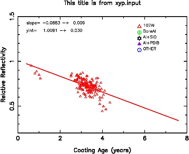 |
| A plot from XYP. We used customized axis labels and plot title using a local xyp.input file. We also explicitly set the axis limits using a local AXIS.LIMITS file. |
If you have generated multiple XYP data files that you wish to view in the same way, an easy run script for doing this is shown below. It assume that you have set up a local AXIS.LIMITS file that will specify the bounds of your plot axes.
% cat PRUN
#!/bin/sh
printf "Usage:  PRUN name_xyp.dat\n"
echo $1 >xyp.input
echo "Age_Years" >>xyp.input
echo "RelRefl" >>xyp.input
echo "Coating Age in Years" >>xyp.input
echo "Relative Reflectivity" >>xyp.input
echo $1" (ALL)" >>xyp.input
#
XYP
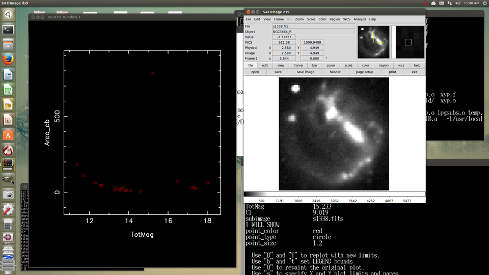 |
| A screen shot made while using XYP to display an image that is associated with a point in the plot that has been identified using the "I" key. Basically, when a piece of information is encountered with the quantity name "subimage", then the value is assumed to be a FITS image name string. This string is fed to the locally open ds9 gui the XPASUBS routine named jun2013_ds9_display_im.f (the user must have opened a ds9 gui prior to running XYP for this to work!). The XY plot (left) was used to isolate a point and the information on that point is shown in the command window (lower-right). As the information set contains the quantity "subimage", then the FITS image associated with this point (named s1338.fits) is plotted (zoomed to fit) in the ds9 window (upper-right). This is somewhat klugy but very effective when needed! |