Wavelength Calibration
The initial goal here is to simply confirm wavelegth ranges and rough
spectral calibrations for each of the four LRS2 spectral channels as
well as the VIRUS units:
  LRS2 arm     Wavelenth Range      Fitted Range Values
  --------     ---------------     ---------------------
    UV           3700   4700          3631.7  4694.4
    Orange       4600   7000
    Red          6500   8420
    Far-Red      8180  10500

    VIRUS        3500   5500
Based on some early work at the telescope, it is clear that we
need some visualization tools that allow us to quickly confirm
the range and ordering of spectral features when we take, for
eaxample, calibration frames with different arc lamps. I have
some more recent (post-2016)
notes LRS2 wavelength calibration.
- Look at an observation+exposure set.
- A rough wavelegnth calibration.
- A better solution.
- Putting things together.
- Using arc lamps.
Look at an observation+exp set.
Both the LRS2 aqnd VIRUS data are taken by specifying and observation
number and an exposure number. After each data set is taken, we might
wish to display the image frames by simply specifying these numbers.
That is the first job we tackle here.
NOTE: This step must be run on a system that has
xpa installed. Below I show the top-level lrs2 data
directory for a night, and an example of using the
ifu_view script to view
some images.
% pwd
/home/sco/LRS2_Nights/20160311/LRS2_images/20160311

% ls
lrs20000601/  lrs20000710/   lrs20000602/
lrs20000101/   lrs20000603/  lrs20000712/
lrs20000102/   lrs20000604/  lrs20000713/
lrs20000103/   lrs20000700/  lrs20000714/
lrs20000600/   lrs20000701/  lrs20000715/

% ifu_view
Usage: ifu_view 603 01 V
arg1 - observation
arg2 - exposure
arg3 - instrument (V,B,R for VIRUS,LRS2-B,LRS2-R)

% ifu_view 603 01 V
The images are zoomed to fit each frame and autoscaled. Note that
most of what ifu_view is doing is constructing image paths. In the
end, the routine ds9_frame_view
is the simples script that displays the images in each of four
ds9 frames. We could horse around with that script and perform
all sorts of scalings, image trasformations, etc... Finally,
I show below a couple of ifu_view runs for some LRS2 sky
flats that Sarah Tuttle and I took at the start (dusk) of
20160311. The sky was dominated by plenty of sunlight and
hence we see numerous solar spectral features.
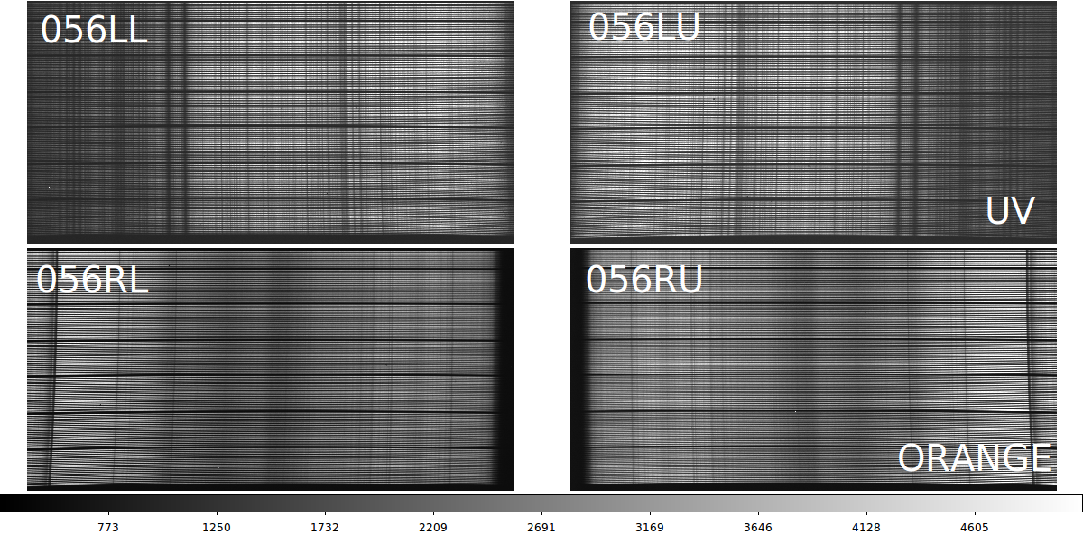 |
The UV (top) and Orange (bottom) arms of LRS2-B from a sky flat
taken on 20160311. The signal is dominated by light from
the Sun, and hence is dominated by the spectral features of
an early G-dwarf star. Even Odewahn could pick out the
strong calcium H,K lines in the UV channel. The approximate
wavelength intervals covered here are:
  LRS2 arm     Wavelenth Range   Spectral Res
    UV           3700   4700        R=1900        (TOP)
    Orange       4600   7000        R=1100        (BOTTOM)
Notice that in the UV images we see the H and K calcium lines and
the solar G-band feature. We'll use these in the next section below.
Note that I added the white figure labels manually
to identify parts of the image names: RL = right detector, Lower
amplifier, and 056 indicates the IFU was in IFUSLOT=056 on the IHMP.
|
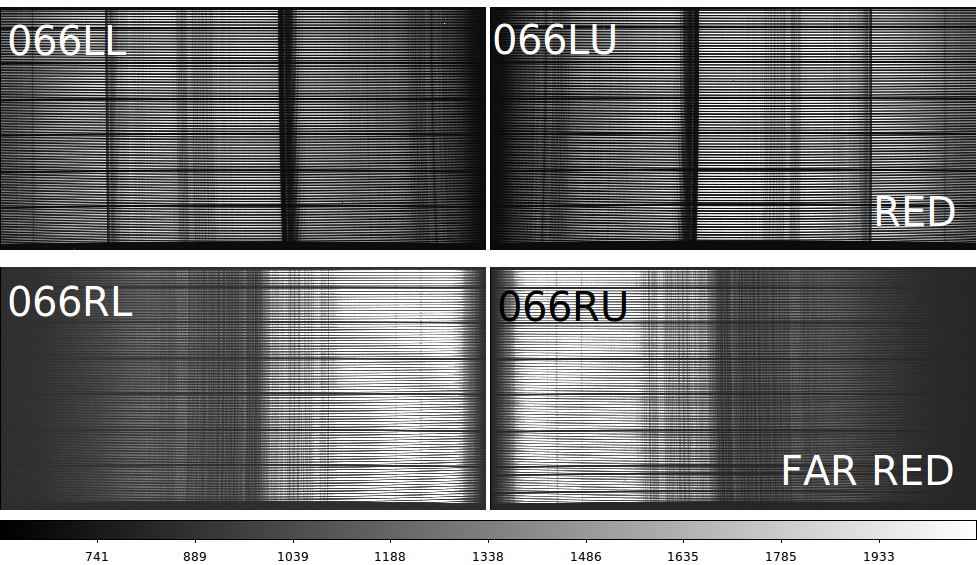 |
The Red (top) and Far-Red (bottom) arms of LRS2-R from a sky flat
taken on 20160311. The signal is dominated by light from
the Sun, and hence is dominated by the spectral features of
an early G-dwarf star. I don't really recognize any solar features
here, but I'm pretty sure the big absorption feature in the Red
arm (top) will turn out to be the telluric absoption feature at
7600 angstroms. The approximate wavelength intervals covered here are:
  LRS2 arm     Wavelenth Range   Spectral Res
    Red          6500   8420        R=1800        (TOP)
    Far-Red      8180  10500        R=1800        (BOTTOM)
|
A rough wavelegnth calibration.
We can use our skyflat images above to get a quick
sense of the wavelength coverage in our LRS2 channels.
The ranges I listed in the above figures are from the
extensive SPIE paper on LRS2 by Chonis etal (need ref here).
We'd like to confirm these ranges and provide a quick and dirty
way to identify or predict the position of any spectral
feature.
Derive a transformation for x (pixels) to y (angstroms).
The fit is made using x,y data from a user-specified input file.
Here is a first guess for features in the LRS2-B channel LL image:

 X_pix   Y_angstroms    feature_name
   1.0     3700.00      blue_end
2128.0     4700.00      red_end
 603.1     3933.66      CaII_K
 678.7     3968.47      CaII_H
1350.3     4306.0       G_band

With the above information I make the table-format input file named LL.dat.

This is really a two step process:

 1) Get the simple  wavelength solution
     % linefit.sh LL_lrs2b.dat
     % mv linefit.explain LL_lrs2b.solution

 2) Use the solution to make a table of wavelengths
     % pix2angs 125.0 LL_lrs2b.dat

To get a wavelength esitmate:
% pix2angs.sh 949 LL_lrs2b.solution
 949.0     4120.1

% cat pix2angs.explain
 949.0     4120.1    (pixels,angstroms)

My final data file for LL:
---------------------------------------
3
X_pix
Y_angstroms
Name
# data
   1.0     3631.00      blue_end
2128.0     4694.00      red_end
 603.1     3933.66      CaII_K
 678.7     3968.47      CaII_H
 949.0     4105.0       Hdelta
1350.3     4306.0       G_band
1414.0     4337.7       Hgamma
1504.0     4382.7       Fe4383
---------------------------------------
A better solution.
To improve the solution we'd like to add some more lines.
Just show one image to make life easier:
/home/sco/LRS2_Nights/20160311/LRS2_images/20160311/lrs20000603/exp01/lrs2/test2
ds9_open 1200 800
ds9_frame_view ./20160311T012519.2_056LL_sci.fits 1

Let's use our solution to predict a new range:
% pix2angs.sh 1 LL_lrs2b.solution
   1.0     3631.1
% pix2angs.sh 2128 LL_lrs2b.solution
2128.0     4694.7

Let's get a list of features for this range:
% speclines.sh
Usage: speclines.sh Hgamma 3700.0 8000.0
arg1 - name of spectral line (can be ANY)
arg2 - minimum allowed output wavelength
arg3 - maximum allowed output wavelength

% speclines.sh ALL 3631.1 4694.7 > my_lines
% cat my_lines
  3727.000  OII_3727
  3934.000  CaII_K
  3968.000  CaII_H
  4101.740  H_delta
  4160.000  CN1_L
  4227.000  Ca4227_L
  4305.000  G_band_L
  4340.470  H_gamma
  4383.000  Fe4383_L
  4455.000  Ca3355_L
  4471.500  HeI_4471
  4531.000  Fe4531_L
  4668.000  Fe4668_L
  4685.680  HeII_4685
  3750.150  H12
  3770.630  H11
  3797.900  H10
  3835.390  H9
  3889.050  H8
  3970.070  Hepsilon
  4101.760  Hdelta
  4340.470  Hgamma

% angs2pix.sh
Usage: angs2pix.sh 6564.2  LL_lrs2b.solution
arg1 - wavelength in Angstroms
arg2 - name of linear solution file

% angs2pix.sh 4305.000 LL_lrs2b.solution
    1348.65     4305.0

I see that my predicted position (X=1348) falls on the G-band feature!
Another way:

% spec_lines_show
Usage: spec_lines_show 1 ./20160311T012519.2_056LU_sci.fits LL_lrs2b.solution 20 cyan ALL
arg1 - ds9 frame number to work in
arg2 - image name
arg3 - wavelength solution file
arg4 - font size for line labels (20)
arg5 - color for line labels (cyan)
arg6 - spectral line group (ALL,Cd,Hg)

% ls
20160311T012519.2_056LL_sci.fits  LL_lrs2b.solution  S/

% spec_lines_show 1 20160311T012519.2_056LL_sci.fits  LL_lrs2b.solution 16 red ALL
Estimated wavelength range = 2128.0     4694.7
Number of lines in your local list = 26 Local.Lines
Here is what we see in our ds9 window:
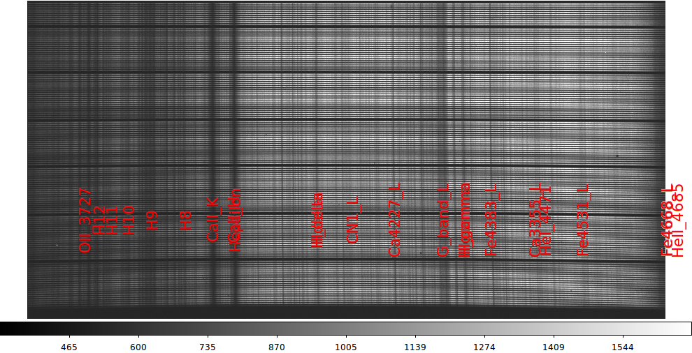 |
Here is a first pass at overplotting our spectral features on top of our LRS2
(LL) image. It is a mess, but with one command line we got a lot of spectral
features that line up with lines in our image. Here is the command line:
% spec_lines_show 1 20160311T012519.2_056LL_sci.fits LL_lrs2b.solution 16 red ALL
Basically, we just gave the frame we wanted to display this in (1), the name of
our image and the name of our wavelength solution file.
|
Not to bad, really. At the end of this run you will notice a
file named "Local.Lines". This file contains the listings
for all of the lines you have plotted. It is easy to edit
this file and re-run your spec_lines_show command again to get
a more cleaned up version of the plot.
I have compiled another set of codes that allow us to edit the
graphical line overlay above. Using the
spec_lines_refit script
we can compile a new list of lines and rederive a wavelength
solution with linefit.sh. This is in an early stage of development,
but a simple example is shown below:
% cat run1
#!/bin/bash
\rm -f Local.Lines
ds9_open 1200 800
ds9_frame_view ./20160311T012519.2_056LL_sci.fits 1
spec_lines_show 1 20160311T012519.2_056LL_sci.fits LL_lrs2b.solution 16 cyan ALL
#
printf "Name of text color for feature to keep (cyan): "
read color
#
spec_lines_refit 1 LL_lrs2b.solution $color Local.Lines

Here is the end of the output from this procedure:
Search for {CaII_K}...................... at X = 606.71 in file Local.Lines
Search for {CaII_H}...................... at X = 672.80 in file Local.Lines
Search for {H_delta}..................... at X = 942.16 in file Local.Lines
Search for {Ca4227_L}.................... at X = 1192.66 in file Local.Lines
Search for {G_band_L}.................... at X = 1348.65 in file Local.Lines
Search for {H_gamma}..................... at X = 1419.59 in file Local.Lines
Search for {Fe4383_L}.................... at X = 1504.64 in file Local.Lines
Search for {Fe4531_L}.................... at X = 1800.62 in file Local.Lines

Number of new lines gathered = 8
   0.4996366  3631.2180176     0.2917482       8   File.X_lam_name
Results from linefit:
     0.4996366       0.0003066    (slope, m.e.)
  3631.2180176       0.3636455    (Y-intercept, m.e.)
     0.2917482                    (Y-sigma)
     8                            (number of fitted points)
We have an improved solution, and the set of 8 overplotted lines
in the figure below now looks pretty good for the LL image in
our LRS2 UV image of our skyflat set.
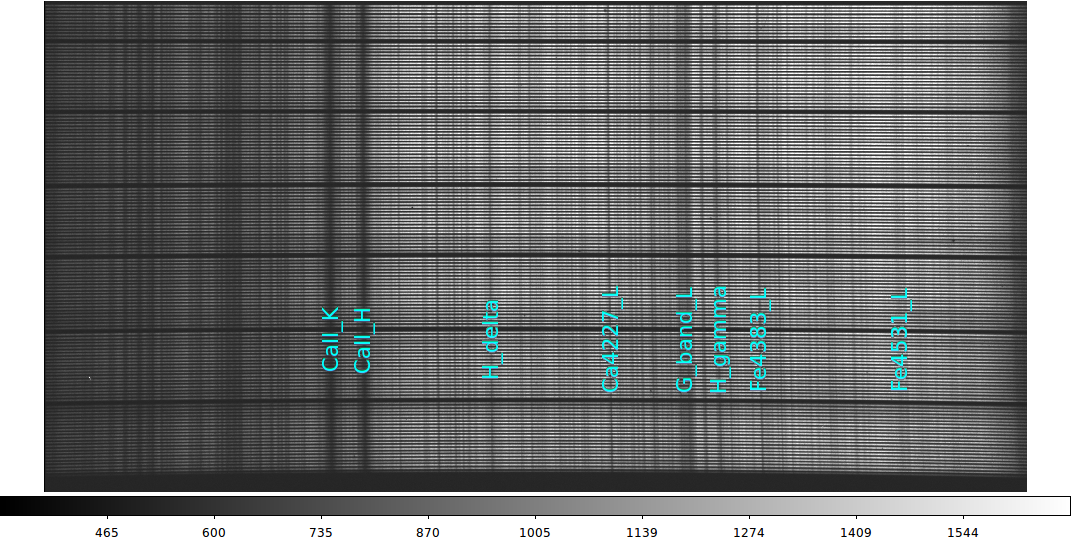 |
Our 8 spectral lines from the LL (LRS2 left amplifier UV) image.
These lines are matched to X pixel positions with:
#
printf "Name of text color for feature to keep (cyan): "
read color
#
spec_lines_refit 1 LL_lrs2b.solution $color Local.Lines
Use the new set of line data (in File.X_lam_name) we use
linefit.sh to derive an improved solution:
% cat linefit.explain
Results from linefit:
     0.4996366       0.0003066    (slope, m.e.)
  3631.2180176       0.3636455    (Y-intercept, m.e.)
     0.2917482                    (Y-sigma)
     8                            (number of fitted points)
|
Below I show our original solution results. I then copy this over
with the revised solution and repeat my exercise above for computing
the spectral range of the image:
Results from linefit:
% cat LL_lrs2b.solution
Results from linefit:
     0.5000380       0.0012129    (slope, m.e.)
  3630.6225586       1.3138450    (Y-intercept, m.e.)
     0.9526117                    (Y-sigma)
     6                            (number of fitted points)

%  mv linefit.explain LL_lrs2b.solution

Let's use our solution to predict a new range:
% pix2angs.sh 1 LL_lrs2b.solution
   1.0     3631.7
% pix2angs.sh 2128 LL_lrs2b.solution
2128.0     4694.4
Putting things together.
Now we'll demonstrate the integration of these tools. But
first, for a lot of the spectral overplotting things we
need wavelegth solution files. Here is a quick fix that
I am using in late Mar2016.
The data files and output solution files made with solar-dominated sky flats are in:
.../projects/Test_Data_for_Codes/T_runs/pix2angs/ex0/

I wrote a little script to copy over available solution files:
% ls
Base.Path  S/

% get_wavesols
Wavelength solution files have been copied to local directory.

% ls
Base.Path  LL_lrs2b.solution  RU_lrs2b.solution  RU_lrs2r.solution  S/
Next, I modified ifu_view to write local files names. When I
run ifu_view to look at images, I produces files with the full
path names:
% ifu_view 604 01 B
Base path = /home/sco/LRS2_Nights/20160311/LRS2_images/20160311
Looking at LRS2-B,  obs,exp = 604 01
Enter any key AFTER ds9 window opens.
DS9 ds9 gs 7f000101:56575 sco
% ls
Base.Path  Frame.2  Frame.4            RU_lrs2b.solution  S/
Frame.1    Frame.3  LL_lrs2b.solution  RU_lrs2r.solution
Finally, as long as I know the name of the appropriate wavelength
file, then I can fit or refit the solution by:
% specfit
Usage: specfit 1 LL_lrs2b.solution ALL
arg1 - ds9 frame number to work in
arg2 - wavelength solution file
arg3 - line group (ALL,Cd,Hg)

% specfit 1 LL_lrs2b.solution ALL
Using the specfit cscript, I have derived the following (rough)
linear wavelength fits:
LRS2B (056)

UV
% cat LL_lrs2b.solution
Results from linefit:
     0.4996366       0.0003066    (slope, m.e.)
  3631.2180176       0.3636455    (Y-intercept, m.e.)
     0.2917482                    (Y-sigma)
     8                            (number of fitted points)

% cat LU_lrs2b.solution
Results from linefit:
    -0.4941828       0.0030003    (slope, m.e.)
  4658.8803711       2.6868012    (Y-intercept, m.e.)
     2.9252040                    (Y-sigma)
     8                            (number of fitted points)

Orange
% cat RL_lrs2b.solution
Results from linefit:
    -1.1904185       0.0028711    (slope, m.e.)
  7012.2968750       3.4209609    (Y-intercept, m.e.)
     5.0703053                    (Y-sigma)
    12                            (number of fitted points)

% cat RU_lrs2b.solution
Results from linefit:
     1.1919098       0.0032778    (slope, m.e.)
  4552.0825195       2.7295449    (Y-intercept, m.e.)
     5.1689687                    (Y-sigma)
     9                            (number of fitted points)


LRS2R (066)
% cat LL_lrs2r.solution

Red
Results from linefit:
     0.9620333       0.0018723    (slope, m.e.)
  6427.4633789       1.1296324    (Y-intercept, m.e.)
     1.0454843                    (Y-sigma)
     3                            (number of fitted points)
% cat LU_lrs2r.solution
Results from linefit:
    -0.9713483       0.0000000    (slope, m.e.)
  8441.3896484       0.0000000    (Y-intercept, m.e.)
     0.0463670                    (Y-sigma)
     3                            (number of fitted points)

Far-Red
% cat RL_lrs2r.solution_sun
Results from linefit:
    -1.2562970       0.0493848    (slope, m.e.)
 10820.7812500      66.2954330    (Y-intercept, m.e.)
    24.7907333                    (Y-sigma)
     6                            (number of fitted points)
% cat RU_lrs2r.solution_dsky
Results from linefit:
     1.1581805       0.0150665    (slope, m.e.)
  8191.0771484      14.7942867    (Y-intercept, m.e.)
    17.8655643                    (Y-sigma)
     6                            (number of fitted points)
% cat RU_lrs2r.solution_sun
Results from linefit:
     1.3057847       0.0448119    (slope, m.e.)
  8170.5102539      33.0752220    (Y-intercept, m.e.)
    21.6579361                    (Y-sigma)
     6                            (number of fitted points)
Some of the red solutions (Far-Red in particular) are crude
due to the lack of prominent lines, especially in the solar-dominated
spectra.
Using arc lamps.
This may seem like "cart before the horse" sort of thing. One
usually starts with an arc lamp when deriving a wavelength
solution. However, in the early commissionong owrk of Feb-Mar
206 we had problems with lamps turning on propoerly (hardware
and softwre?), light guide insertion, FCU insertion (FCU = Field
Calibration Unit), etc.... Hence, I started above with something
that I was pretty sure of: sunlight. Now that we have rough
wavelength solutions for each LRS2 channel (i.e. L and U amplifiers in
the UV, Orange, Red, and Far-Red arms) we can better go through the
arcs taken on 20160311. Here are some distilled notes from the
log for the cals taken that night. We took the cals just after
the sky flats from above were taken (while the TO was stacking M1):
Breakdown of cals and flats from 20160311
(all in observation=101,  exposure= 00-07)

exp00  = Hg lamp on slider a for 120 seconds with red light guide
         signal in UV,Orange,Red,Far-Red
         Hg_B_101_00.png
         Hg_R_101_00.png

exp01  = Hg lamp on slider a for 10 seconds with blue light guide
         signal in UV,Orange, weak in Red, none in Far-Red
         Hg_B_101_01.png
         Hg_R_101_01.png

exp02  = Cd lamp on slider b for 240 seconds with red light guide
         No UV, few Orange; good lines in Red and Far-Red
         Cd_B_101_02.png
         Cd_R_101_02.png

exp03  = Cd lamp on slider b for 60 seconds with blue light guide
         No UV, some weak Orange;  No Red or Far-Red
         Cd_B_101_03.png
         Cd_R_101_03.png

exp04  = Qth lamp on slider b for 8 seconds with red light guide
         cutoff in UV, good signal in Orange, Red, Far-Red

exp05  = Qth lamp on slider b for 30 seconds with blue light guide
         cutoff in UV, good signal in Orange, cutoff in Red, non Far-Red

exp06  = ldls lamp on slider ldls for 1.0 seconds with red light guide
         cutoff in UV, signal in Orange, cutoffs in Red, Far-Red

exp07  = ldls lamp on slider ldls for 5 seconds with blue light guide
         signal in UV,Orange;  cutoff in Red, non Far-Red

NOTE: We need a clear description of the "slider"
and "light guide" terminology.
I will use specfit with the Hg and Cd lamps (when signal is available) to
derive wavelength solutions for the following:
Wavelength File    Channel  Arm (amp)

LL_lrs2b.solution     B     UV (lower)
LU_lrs2b.solution     B     UV (upper)
RL_lrs2b.solution     B     Orange (lower)
RU_lrs2b.solution     B     Orange (upper)

LL_lrs2r.solution     R     Red (lower)
LU_lrs2r.solution     R     Red (upper)
RL_lrs2r.solution     R     Far-Red (lower)
RU_lrs2r.solution     R     Far-Red (upper)
Back to VIRUS_LRS2 Tools page