tim_* (Compute Test Images)
Updated: Jul17,2020
In March2014 I began writing various image processing modules using python.
To generate test input for some of these code I have written a suite of Test
Image (tim) codes. These are gfortran codes in the OTW environment. Unless
otherwise noted, these test images have the output size of 256x256 pixels
written as floating point (BITPIX=-32).
tim_stripes.sh
This generates an image where each column of pixels has
a fixed value. Hence we are generating an image of "stripes".
The arguments to tim_stripes are fed in a pars.in file. This
file is generated by the script tim_stripes.sh. The arguments
are the start and end stripe values, and the name of the output
image to be generated.
% tim_stripes.sh 1 256 R.fits
The image generated by this called, named R.fits, is
shown in the figure below. The first column (x=1)
has a values of I=1, and the last column (x=256) has
a value of I=256. As an aside, I show below the commands
I use to generate this image. The command named "jpeg256.py"
is a python code that takes 3 (RGB) images, and generates
an output jpeg image file. Actually, the whole genesis
of the tim series of tasks lies in developing python
codes like this. For now, we simply need to know that
"jpeg256.py" takes the 3 images from tim_stripes runs,
and generates a grey-scale image.
To create the figure below:
#
tim_stripes.sh 1 256 R.fits
tim_stripes.sh 1 256 G.fits
tim_stripes.sh 1 256 B.fits
python jpeg256.py
mv sco.jpeg test_stripes.jpeg

It is useful to note here that I used the ImageMagick
"display" command to view the test_stripes.jpeg file:

# display test_stripes.jpeg
To add the yellow test label seen in the figure below
I just left-clicked in the display window. I then selected
from the menu "Image Edit > Annotate". When doe with the
labeleing I used the "File > Save" option to save the updated
jpeg file. This is a rather klugy, but easy and diret way to make
labeled images.
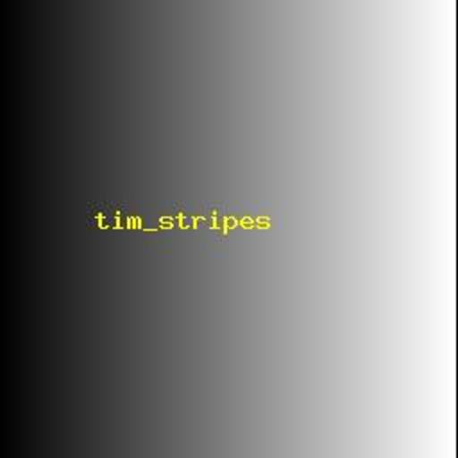 |
| An example of an image generated with tim_stripes.
As descibed above, I used the useful command "display tim_stripes.jpeg"
to display this jpeg (from the command line). I then used a few
simple cursor-based command to add the yellow text label in the
center of the image.
|
tim_circle.sh
This generates an image of a circle. The brightness distribution
with in the circle is defined radially using arguments 4 and 5. The
position and size of the circle are also input values. I used this
simple code to generate red, green and blue images that were then
combined with the "jpeg256.py" code to create the color figure shown
below.
#
tim_circle.sh 128 100 90.0 256 200 R.fits
tim_circle.sh 100 160 90.0 256 200 G.fits
tim_circle.sh 160 160 90.0 256 200 B.fits
python jpeg256.py
convert sco.jpeg -resize 512x512 tim_circle_1.jpeg

 I use "convert" to make the image larger (512x512).

Here are the arguments fed to tim_circle.sh:
  arg1 - Xo of circle
  arg2 - Yo of circle
  arg3 - Ro, radius of circle
  arg4 - I value at R=0
  arg5 - I value at R=Ro
  arg6 - name of output test image
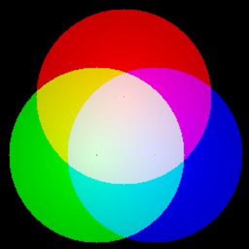 |
| Color image generated with three (RGB) images from
tim_circle.sh. For each circle (each a different color) the center
of the circle has I=256 and the edge of the circle has I=200. The
overlap regions are all white, since the color ratios from each image
are equal for each color.
|
One of the reasons for writing tim_circle was to illustrate not
only how color images are generated, but how brightness is controlled
in a color image. Below I show a script used to change the relative
colors and brightnesses of the above figure. The resultant figure is
displayed below.
% cat R2_2
#
tim_circle.sh 128 100 90.0 256 100 R.fits
tim_circle.sh 100 160 90.0 256 175 G.fits
tim_circle.sh 160 160 90.0 256  40 B.fits
jpeg256.py
convert sco.jpeg -resize 512x512 tim_circle_2.jpeg
display tim_circle_2.jpeg &
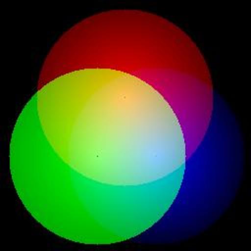 |
| Color image generated with three (RGB) images from
tim_circle.sh. The variation in pixel values in the constituent
RGB images control not only the resultant color, but also the brightness
in the output image.
|
Back to SCO CODES page