A very practical use for point_selector is to view a parameter space and derive statistics for all or some of the data points. First I show below some of the critical files: the parlab file that gives the short parameter names and then longer, more explanatory names, and the first few lines of a typical data prortion of the table file.

Basename of the table file is:  acm_bias_singles
To make the local directory less cluttered I use: ../Jul1-22_2020/acm_bias_singles

% cat ../Jul1-22_2020/acm_bias_singles.parlab
bmean    Mean BIAS signal (adu) 
bme     mean error about mean BIAS signal (adu) 
bsig     Standard deviation about mean BIAS signal (adu) 
npix     Number of pixels for BIAS determination 
d2000    Days since Jan1,2000 
djan1    Days since Jan1 
uth      UT in hours 
temp     Ambient Temperature (deg C) 
year     Year 
mon      Month number 
day      Day number (in month) 
image    acm image basename 

% head -5 ../Jul1-22_2020/acm_bias_singles.table 
# data
  1389.8717 0.0353 21.2071 361201 7486.437500 182.937683 22.50447 25.84 2020 07 01 20200701T223016.1_acm_sci 
  1390.0443 0.0353 21.2196 361201 7486.437988 182.937820 22.50758 25.84 2020 07 01 20200701T223027.3_acm_sci 
  1390.0308 0.0353 21.2435 361201 7486.437988 182.937943 22.51058 25.84 2020 07 01 20200701T223038.1_acm_sci 
  1390.0020 0.0351 21.1239 361201 7486.437988 182.938065 22.51361 25.84 2020 07 01 20200701T223049.0_acm_sci 

% point_selector --help    

The first step in this process is to creat the plot of our desired parameter space.

% point_selector ../Jul1-22_2020/acm_bias_singles uth bmean N  

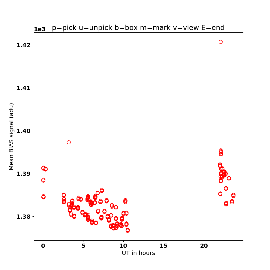The initial plot we generate with point_selector: % ls matplotlibrc % point_selector ../Jul1-22_2020/acm_bias_singles uth bmean N The file matplotlibrc is simply present to reformat some of the plot properties. If it were not present, then the axis labling would not be bold face and would be smaller in size. Next we can use the usual show() icons atthe top of the plot to zoom into different areas. I want to know the mean statistics of the clump of points around X=22 hours.

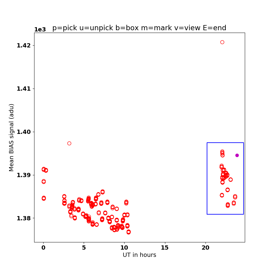We have used the zoom icon (the one that looks like a magnifying glass). I used it to zoom into the clump at X=22 hours. I then hit the "b" key yo mark all of the points in the zoomed-in region. Lastly I went back to the original plot view using the home icon (the one that looks like a house). We should note that the small purple dot is made to indicate that we have marked the points in the zoomed in box. After I use the "E" key to end the plotting process, we in our local working directory: % ls Last.BoxLims matplotlibrc xyf.in The Last.BoxLims file records the axis ranges we last used, and the xyf.in records which points were marks and unmarked.

A list of the recognized key-strokes and there resultant actions is given below.

The key entries that are recognized by point_selector:
  key    function 
   v     View (in ds9) the image associate with the selected point 
   p     Select the point closest to the cursor    (uses pointclean.sh)
   u     Deselect the point closest to the cursor  (uses pointclean.sh) 
   b     Mark all points in the current box as selected 
   m     Simply record the cuurent marked position of the cursor 
   E     End the marking operation 

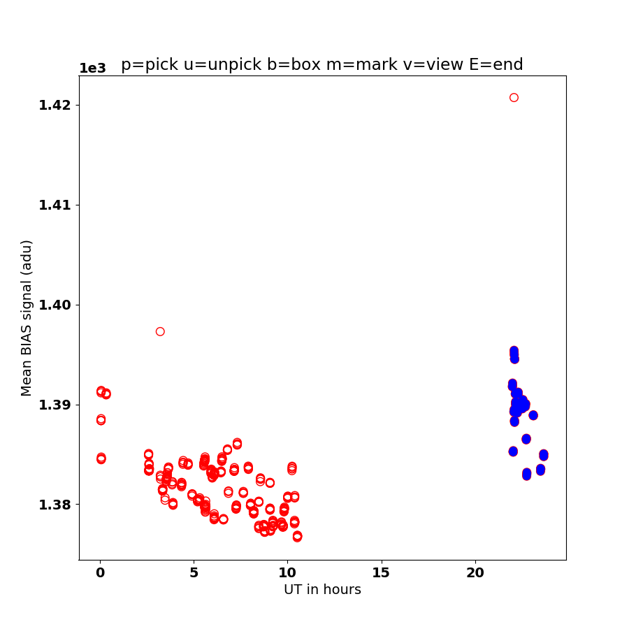Here we have rerun the point_selector code and we have answered "N" to the first question about deleting files from the previous run. *** There are files from a previous run. Do you want to delete them? (Y/N): N In this way, our marked points in the box we zoomed into are now plotted as blue circles.

The lat step is to use the identified "marked" points in the xyf.in file to compute some simple statistics using the point_selector_stats routine. We can specify the axis we are interested and whether we wish to know the statistics of the unmareld (0) or marked (1) points in xyf.in.

Usage: point_selector_stats.sh xyf.in X 0 N 
arg1 - name of xyf.in-type file (usually xyf.in) 
arg2 - Axis to to analyzed (X or Y) )  
arg3 - flag value to be pulled (usually 0 or 1)  
arg4 - run in debug/verbose mode (Y/N)  

% point_selector_stats.sh xyf.in Y 1 N  
1389.03210   1389.60120      3.17560      0.32754       94   (mean,median,sig,me,n)

As of Jul2020 I have added a section to point_selector that compute the X and Y statistics for the marked and unmarked points. The results are shown to the user at the end of a point_selector run.