This page probably falls into the overkill category, but it demonstrates a number of useful things. As ilustrated in the figure below, line_resid compute the normal distance from a point (Xo,Yo) to a line having the equation y=ax+b. To run this simple demo routine:

 
% line_resid.sh 1.3 2.5  2.0 -3.5 
% line_resid_plot.py  
% display line_resid.png  

Usage: line_resid 1.05 0.05 3.0 2.0       
arg1 - line slope, a (where y=ax+b)       
arg2 - line Y-intercept, b (where y=ax+b) 
arg3 - Xo (x position of residual point)  
arg4 - Yo (y position of residual point)  

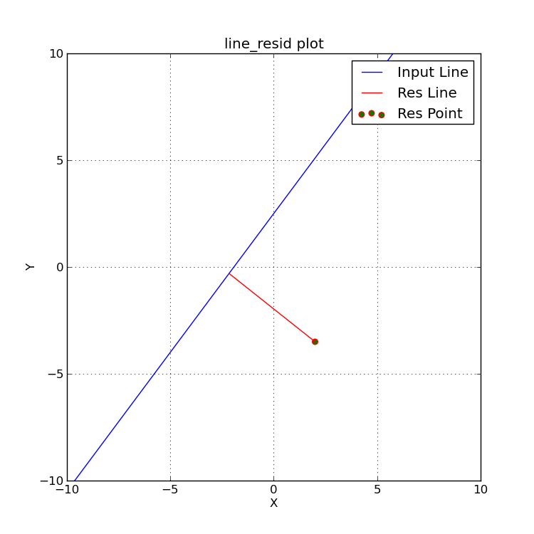The blue line represents the input line (y=ax+b). The green point is (Xo,Yo), the point for which we want to compute the perpendicular distance (residual) to the line. Here is how I made and inspected this plot: % line_resid.sh 1.3 2.5 2.0 -3.5 % line_resid_plot.py % display line_resid.png

Actually I will rarely use line_resid in practice. The routine that preforms the work, and is used in various OTW routines, is in OTWLIB:line_subs/xyline_res.f, and typical call would be something like:

      call xyline_res(a,b,xo,yo,databack,log)
where the "answers" are returned in databack:

c**************************************************************************
      dimension databack(20)
c Derive line equation for perpendicular residual segment.
c databack(1) = residual
c databack(2) = alpha, slope of residual segment line
c databack(3) = beta,  y-int of residual segment line
c databack(4) = xlo, x of line-residual intersection
c databack(5) = ylo, y of line-residual intersection
c databack(6) = xo, x of point for which residual is computed
c databack(7) = yo, y of point for which residual is computed

Continuing in the spirit of overkill, I show the simple python plotting code that I use to make the figure above. The code is:

 
 .../otw/src/line_resid/plot_py/line_resid_plot.py.

 
 
#!/usr/bin/python
print "\nUsage: line_resid_plot.py\n" 
   
# Setup to read the name of the input file 
from sys import argv
script_name = argv

# Numpy is a library for handling arrays (like data points)
import numpy as npsubs

# Pyplot is a module within the matplotlib library for plotting
import matplotlib.pyplot as plt

#==================================================
# Open the files for read-only 
f = open('line1.dat', 'r')
# initialize some variable to be lists:
x1 = []
y1 = []
n1 = 0 
i = 0
while True:
 if i < 20:
   line = f.readline() 
   p = line.split()
   x1.append(float(p[0]))  
   y1.append(float(p[1]))
 else:
   break
 i=i+1
n1 = i 
f.close() 
#==================================================

#==================================================
# Read the line2.dat file 
f2 = open('line2.dat', 'r')
x2 = []
y2 = []
n2 = 0
for line in f2:
    p = line.split()
    x2.append(float(p[0]))  
    y2.append(float(p[1]))
    n2 = n2+1
f2.close() 
#==================================================

# Create the numpy arrays 
xv1 = npsubs.array(x1)
yv1 = npsubs.array(y1)

###################################################
# Set the physical size 
xpsize = 7.5 
ypsize = 7.5 
###################################################

#===========================================================
# Plot the input line (line1) data 
fig = plt.figure(figsize = (xpsize,ypsize))

# Set up the axes 
xlo="-10"
xhi="+10"
ylo=xlo
yhi=xhi
xlim1 = float(xlo)  
xlim2 = float(xhi) 
ylim1 = float(ylo) 
ylim2 = float(yhi) 
plt.xlim(xlim1,xlim2)
plt.ylim(ylim1,ylim2)

# Plot the data 
plt.scatter(x2[0], y2[0], s=30, facecolor="green", edgecolor="red", label="Res Point") 

# Plot the input line 
plt.plot(x1, y1, c='blue', linestyle='-', label='Input Line') 

# Plot the residual line 
plt.plot(x2, y2, c='red', linestyle='-', label='Res Line') 

# add some fancy touches 
plt.grid(True) 
plt.legend() 

# label the axes 
plt.title("line_resid plot")
plt.xlabel("X")
plt.ylabel("Y")

#plt.show()
plt.savefig('line_resid.png')
print '\nUse to view your plot:\ndisplay line_resid.png\n'
#===========================================================