 |
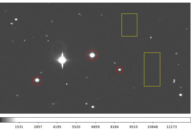
| FIGURE 1: A sample image marked up with ID. |
ID (Image Display) displays an image with ds9+xpa and allows the user to create and store markers. These markers may, for example, be used by down-stream codes to identify elliptical (galaxy) apertures, a column of mirrors in a hexburst image, or a set of stars to be used for constructing a mean stellar PSF for the image.
Go to the id test directory (use gotr) and choose a subdirectory for testing. In the simplest mode, after invoking ID, just type in the name of the FITS image you want to view and mark up.
%  pwd
/home/sco/sco/projects/Test_Data_for_Codes/T_runs/id/generic
%  ls
S/
%  S/GRAB

You can now run ID
Local test image = m51.fits
.  ..  m51.fits  S
%  ID
 No local file: id.input

Enter name of input file to use:  m51.fits

 ANSWER QUERIES UNTIL DONE
At the end of the ID, there may be a number of files present but the most important ones are:
id.objects  == an ASCII file storing the marker info
               in formats that SCO codes understand

m51.info    == the *.info for the image you processed. This
               file will contains the ID marker info (the
               id.objects) and other output files as you
               process them with other codes.
I usually use ID to mark objects to be photometered. Below is a sample image, an image that is dumped by ID to a JPEG file while it is running!
|
| FIGURE 1: A sample image marked up with ID. |
Sometimes, I run ID from other programs and do not want to always manually specify the name of the input image. If you create a local file called "id.input" that contains the name of the image file to be processed, then the interactive query is skipped. Finally, I have a little script called "run_id" that will build "id.input" and run ID. To use it just type soemthing like:
run_id name_of_image.fitsThis will get you pretty much anything you want for image mark-up. Maybe not.
I am also writing a number of scripts for catalog production, matching, mergeing, etc... One very useful thing is to be able to overplot the catalog sources on a ds9 display of an image. In SCOLIB.xpadisp.f I have a lot of tools for constructing region files. However, I am finding that python and bash scripting may, again, prove more versatile and easier t control than f77. This seems like a good time to summarize properties of the region file formats. I have used ds9 to make the figure below that uses a variety of region marker properties. I then generated the region file for this set and display that file just below the figure.
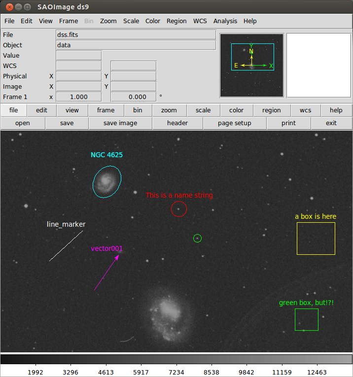 |
| FIGURE 2: A variety of ds9 region markers. |
Below I show three versions of saving the region files for the ds9 markers above.
% cat ds9_image.reg
# Region file format: DS9 version 4.1
# Filename: dss.fits
global color=green dashlist=8 3 width=1 font="helvetica 10 normal roman" select=1 highlite=1 dash=0 fixed=0 edit=1 move=1 delete=1 include=1 source=1
image
circle(591,674,8.0682613)
circle(553.00319,734.00065,15.91123) # color=red text={This is a name string}
box(830.50069,674.4987,76.999999,64.999999,3.7329666e-07) # color=yellow text={a box is here}
box(811.50235,509.00281,47.000001,44,3.7329666e-07) # text={green box, but!?!}
ellipse(406.99729,788.99714,26.000001,34.000001,328.65585) # color=cyan text={NGC 4625}
line(290.99788,628.00014,358.00043,690.00181) # line=0 0 color=white text={line_marker}
# vector(381.99825,569.99892,86.277293,55.388852) vector=1 color=magenta text={vector001}


% cat ds9_fk5_sex.reg
# Region file format: DS9 version 4.1
# Filename: dss.fits
global color=green dashlist=8 3 width=1 font="helvetica 10 normal roman" select=1 highlite=1 dash=0 fixed=0 edit=1 move=1 delete=1 include=1 source=1
fk5
circle(12:41:24.062,+41:13:10.87,13.7166")
circle(12:41:29.923,+41:14:51.92,27.0502") # color=red text={This is a name string}
box(12:40:47.979,+41:13:17.35,130.905",110.52",0.871148) # color=yellow text={a box is here}
box(12:40:50.513,+41:08:35.56,79.9032",74.8136",0.871148) # text={green box, but!?!}
ellipse(12:41:52.063,+41:16:21.57,44.2018",57.8105",329.527) # color=cyan text={NGC 4625}
line(12:42:09.142,+41:11:44.62,12:41:59.205,+41:13:31.92) # line=0 0 color=white text={line_marker}
# vector(12:41:55.295,+41:10:08.57,146.677",56.26) vector=1 color=magenta text={vector001}

% cat ds9_fk5_fp.reg
# Region file format: DS9 version 4.1
# Filename: dss.fits
global color=green dashlist=8 3 width=1 font="helvetica 10 normal roman" select=1 highlite=1 dash=0 fixed=0 edit=1 move=1 delete=1 include=1 source=1
fk5
circle(190.35026,41.219686,13.716598")
circle(190.37468,41.247756,27.050184") # color=red text={This is a name string}
box(190.19991,41.221486,130.90528",110.52013",0.871148) # color=yellow text={a box is here}
box(190.21047,41.143211,79.903228",74.813627",0.871148) # text={green box, but!?!}
ellipse(190.46693,41.272658,44.201786",57.810532",329.527) # color=cyan text={NGC 4625}
line(190.53809,41.195728,190.49669,41.225533) # line=0 0 color=white text={line_marker}
# vector(190.4804,41.169047,146.67732",56.26) vector=1 color=magenta text={vector001}
   z1 = bkg + a1*sigma
   z2 = bkg + a2*sigma

For PFC galaxies, I typically use  a1=-1.0 , a2=100.0
I find that these auto-scaled levels tend to save time by avoiding a lot of recourse to the Scale option in ds9.
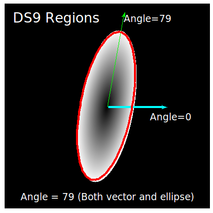 |
| FIGURE 3: An example of Angle for ellipse and vector regions in ds9. |