Here are some early working notes about running trs_solve_1.
This work done originally in: /home/sco/shuf_examples/het_eng/shuf1
This file originally: /home/sco/shuf_examples/het_eng/shuf1/S/README.trs
Usage: trs_solve_2 file1.xy file2.xy 2 1.35 -30.0 N
arg1 - file with XY to be transformed to (Defines system)
arg2 - file with XY to be transformed
arg3 - Point number defining origin (1)
arg4 - scale factor (can also be "Q" or "S")
arg5 - Rotation angle in degrees (can be "Q" or "S")
arg6 - Reflection axis (X,Y, or N for none)
NOTE: Q=query S=solve
NOTE: local PointNames file must be present
For problem here:
file1 = XY in the acm system (system to be transformed to)
file2 = the IHMP coordinates
Must have a PointNames file
# data
056 -49.8 -148.7 741.8 213.3
066 49.8 -151.3 744.5 581.5
555 3.3 -73.2 452.6 402.6
600 -35.0 10.1 148 254.8
000 0.0 0.0 183.3 386.3
I split the above table into 3 files:
% cat PointNames
056
066
555
600
000
% cat acm.xy
# acm measure pre-Dec2017
# data
741.8 213.3
744.5 581.5
452.6 402.6
148.0 254.8
183.3 386.3
% cat ihmp.xy
# IHMP positions
# data
-49.8 -148.7
49.8 -151.3
3.3 -73.2
-35.0 10.1
0.0 0.0
--------------------------------------------------------
file1 = acm.xy (these define the system)
file2 = ihmp.xy (these will be transformed)
To solve:
file1 file2 p scale rot flip
trs_solve_2 acm.xy ihmp.xy 3 3.6913 S N
To view informative plots:
To see the original data:
trs_2plot file1_original.xy file2_original.xy
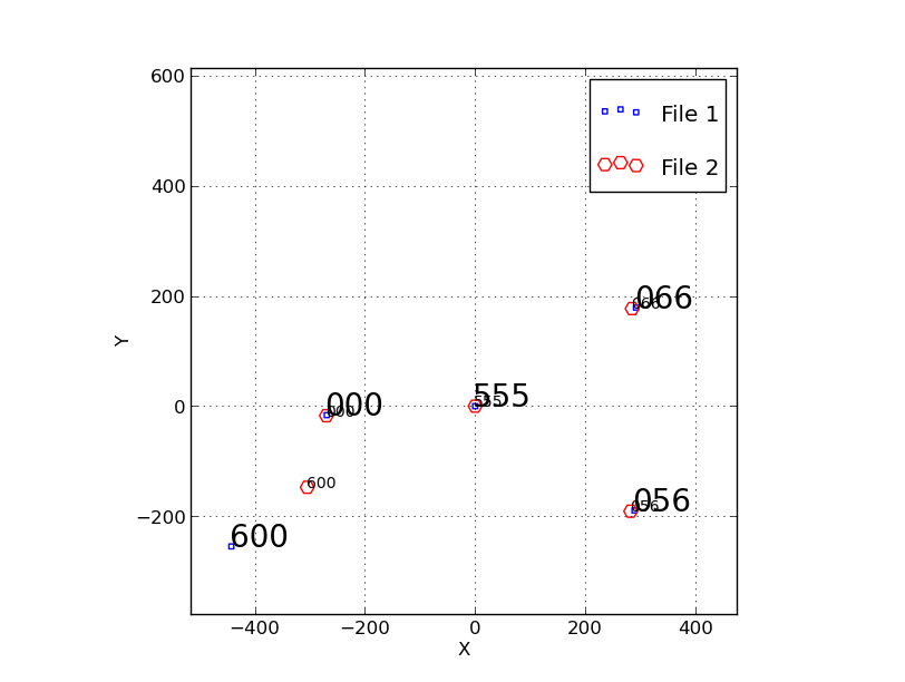
Plot1.png ==
The small blue squares (labeld as File 1 in the legend) are the original
acm positions in units of pixels. This is the system to want to transform to.
The red circles (labeld as File 2 in the legend) are the IHMP (fplane.txt)
positions. It is the X,Y=0,0 in this system that we wish to transform to the
acm system. We see that no flip is required, and we see that the X,Y values
in pixels (acm) cover a larger spatial range than those in arcseconds (IHMP)
since the acm plate scale is 0.2709 arcsec/pix.
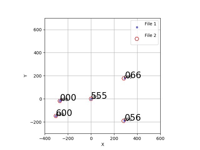
To see after translation (or both sets):
trs_2plot file1_trans.xy file2_trans.xy
To see after file2 is scaled:
trs_2plot file1_trans.xy file2_scal.xy
To see after file2 is scaled and rotated:
trs_2plot file1_trans.xy file2_rotate.xy
**** Looks like the "600" point is discrepant.
 |
Here is the solution I get uisng 000,056,066.555, and 600. These
are IHMP. LRS2B, LRS2R, BIB, and HPF. The command line was:
% trs_solve_2 acm.xy ihmp.xy 3 3.6913 S N
% trs_2plot file1_trans.xy file2_rotate.xy
% trs_plot.py Style.file -50 50 -50 50 SHOW
Tere appears to be some misunderstanding about what point 600 is.
|
Looks like I had a typo in my acm.xy data file for 600. Here is the correct run results:
[astronomer@mcs shuf1]$ cat Final_Residuals.List

Residuals List, coordinates are in units of file: acm.xy
X1,Y1  = original coordinates from acm.xy
X2,Y2  = coordinates from ihmp.xy transformed to the acm.xy system
# List of XY residuals from xy_tranrot_res.sh
  line       X1        Y1           X2        Y2           dX        dY          Res       Res_norm
    1     741.800   213.300      735.304   212.422        6.496     0.878        6.555      1.7418
    2     744.500   581.500      737.264   580.195        7.236     1.305        7.353      1.9537
    3     452.600   402.600      452.600   402.600        0.000     0.000        0.000      0.0000
    4     148.000   254.800      148.117   254.868       -0.117    -0.068        0.135      0.0360
    5     183.300   386.300      182.708   384.810        0.592     1.490        1.603      0.4260

The mean residuals statistics were:
RMS of X residuals (file1-file2) = 3.693
RMS of Y residuals (file1-file2) = 0.724
Number of residuals points used  = 5

To get plot of final transform:
% trs_2plot file1_trans.xy file2_rotate.xy

    trs_plot.py Style.file -50 50 -50 50 SHOW         # does not work on mcs
    trs_plot.py Style.file -400 600 -300 700 HARD

Now I get a very nice plot and solution.

Fianlly, to make the transformation using the solution file and a data
file having only the IHMP oriigin:

# IHMP origin point
# data
    0.0    0.0

[astronomer@mcs A1]$ trs_apply a.xy TRS.final Y
# data
  182.708	  384.810

The acm position in the wiki is:
IHMP - 183.3 386.3                   # Very close to my solution value!!!
 |
Here is the solution I get uisng 000,056,066.555, and 600. I have corrected
the typo I made for 600 in the acm.xy file.
% trs_solve_2 acm.xy ihmp.xy 3 3.6913 S N
% trs_2plot file1_trans.xy file2_rotate.xy
% trs_plot.py Style.file -50 50 -50 50 SHOW         # does NOT work on mcs
% trs_plot.py Style.file -400 600 -300 700 HARD     # works fine on mcs
This solution is a good one. One odd point: the show() plotting fails when I run as astronomer, but if I
run from my sco account on mcs the show() facility works just fine. Argh!
|
Fianlly, I made a script to do everythin from one file:
#!/bin/bash
debug="N"

# Sampel file:
# 056     -49.8 -148.7   741.8 213.3
# 066      49.8 -151.3   744.5 581.5
# 555       3.3  -73.2   452.6 402.6
# 600     -35.0   10.1   148.0 254.8

# Check command line arguments
if [ -z "$1" ]
then
 printf "Usage: find_ihmp_on_acm Data.ALL\n"
 printf "arg1 - input data file (name X,Y_ihmp X,Y_acm) \n"
 exit
fi
if [ $1 = "--help" ]
then
 show_help find_ihmp_on_acm
 exit
fi

fdat="$1"

# Cut out header
data_strip $fdat
mv data_strip.table B0

# Get the names
awk < B0 '{ print $1 } ' > PointNames

# Get ihmp data
printf "# IHMP positions \n# data\n" > ihmp.xy
awk < B0 '{ print $2 " " $3 } ' >> ihmp.xy

# Get acm data
printf "# acm positions \n# data\n" > acm.xy
awk < B0 '{ print $4 " " $5 } ' >> acm.xy

# Run the solution
#            file1  file2   p  scale  rot flip
trs_solve_2 acm.xy ihmp.xy  3  3.6913  S   N

printf "# IHMP origin \n# data\n 0.0 0.0 \n" > a.xy
printf "\n**** Now Computing IHMP Origin on acm **** \n"
trs_apply a.xy TRS.final Y

printf "\n\nPlot the results? Y/N: "
read ans
if [ $ans = "Y" ]
then
 printf "I am running: \ntrs_plot.py Style.file -400 600 -300 700 HARD\n"
 trs_plot.py Style.file -400 600 -300 700 HARD
 trs_plot.py Style.file -400 600 -300 700 SHOW
fi
Back to calling page