As described in the main page of this document, we manually construct a file containing the positions of several detectors in the IHMP system of the fplane.txt file (in units of arcseconds) and in the acm camra system (in units of acm pixles).

% cat Data.ALL
# IHMP-acm positions after Sep2018 FPA take-down
# name     X,Y_ihmp         X,Y_acm      X,Y_acm _prev
# data
555       0.7  -73.1     455.0  398.7    455.0  398.7
600     -39.9   9.97     148.7  250.3    148.7  250.3
056     -50.0 -150.0     738.6  211.6    738.6  211.6
066      50.0 -150.0     739.7  577.3    739.7  577.3

The routine find_ihmp_on_acm is used to process this file and derive estimates of acam_x_origin and acam_y_origin. Basically, we derive the linear tranformation that will convert (X,Y) in the IHMP system (from the fplane.txt file) to (X,Y) in the acm system. Using this solution we convert (X,Y)_ihmp = 0,0 to the acm system to produce (X,Y)_acm = acam_x_origin,acam_y_origin. We would run this routine as:

 

%  find_ihmp_on_acm Data.ALL   
Newly derived IHMP center in units of acm pixels: 
acam_x_origin  =  185.251 -+ 0.302 
acam_y_origin  =  397.199 -+ 1.711
See file Final_Residuals.List for more detail.

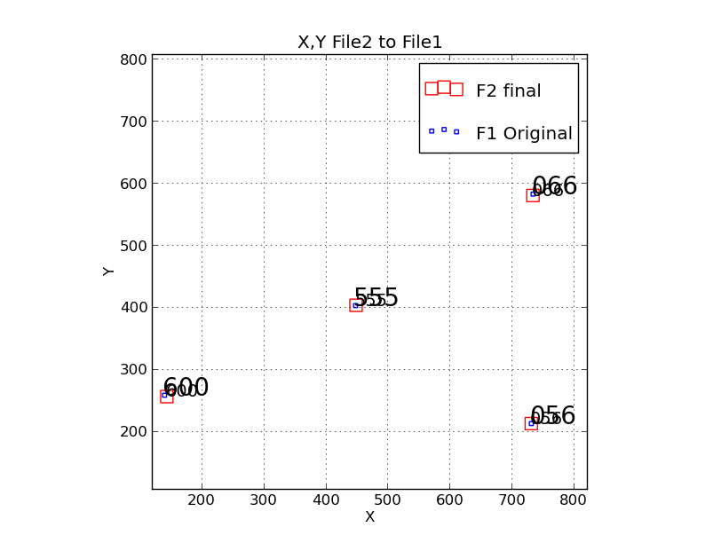The IHMP to acm fit made with the positions (acm coordinate frame in pixel units) for 056 (LRS2-B), 066(LRS2-R), 555(BIB), and 600(HPFacq). In this case the small blue squares are the original acm positions. The larger red squares are the IHMP positions transformed to the acm system using the results from a run of the trs_solve_2 routine. These results are contained in the local file named TRS.final. Below is the the command line call to run the routine find_ihmp_on_acm: % find_ihmp_on_acm Data.ALL # the command line Newly derived IHMP center in units of acm pixels: acam_x_origin = 185.251 -+ 0.302 acam_y_origin = 397.199 -+ 1.711

As a sanity check we began using a simple graphical derivation of the (acam_x_origin,acam_y_origin) point on the acm. This method depends only on the radius of each imageing device (LRS2-R,LRS2-B,BIB, and HPFacq) fron the IHMP cenetr (derived from the fplane,txt file) and the centers of these imaging devices as determined with bright stars. A description of this graphical method is presented and the routine for implementing is shown below.

% acm_xy_graphical Data.ALL  
Result from acm_xy_graphical:  
acam_x_origin  =  185.10  -+  2.08   (acm pixels)  
acam_y_origin  =  397.59  -+  2.08   (acm pixels)  
 

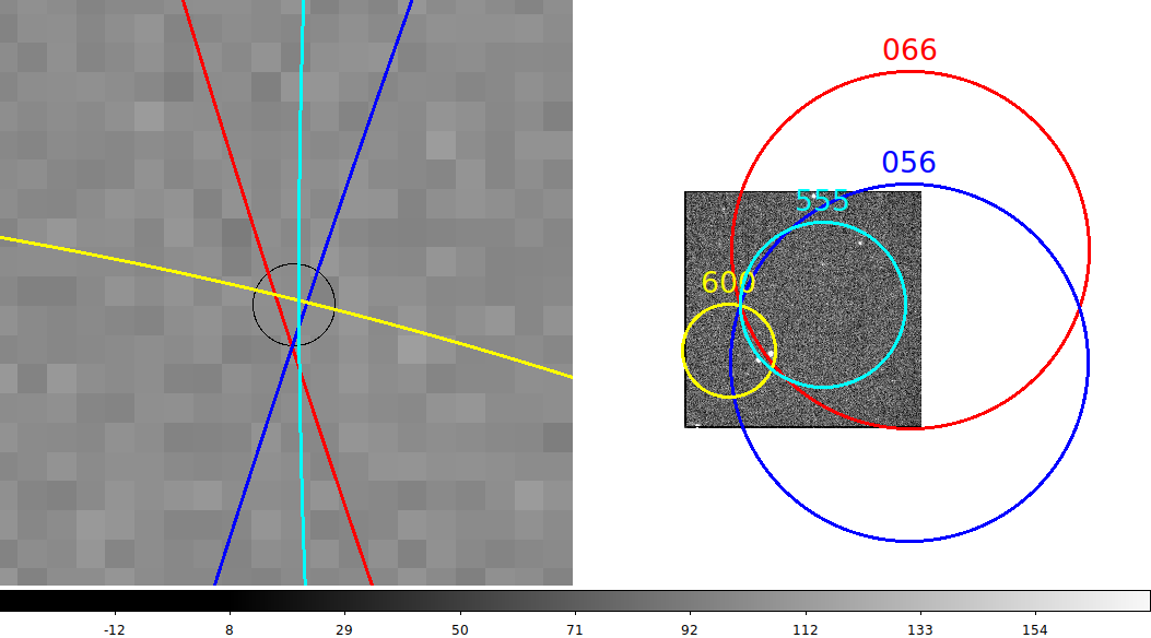The left panel shows the overlap of the radial zones for the 056 (LRS2-B), 066(LRS2-R), 555(BIB), and 600(HPFacq) detectores overplotted on a random acm image. This was made with the command: % acm_xy_graphical Data.ALL Result from acm_xy_graphical: acam_x_origin = 185.10 -+ 2.08 (acm pixels) acam_y_origin = 397.59 -+ 2.08 (acm pixels) The black circle represents a "visual fit" to the overlapping zones. The cenetr of this circle represenst the position of the IHMP center in the acm coordinate system. The right panel shows the full field view taht allows th reader to see each labeled radial zone.