View a histogram starting with ds9_imstats.
Last updated: Oct17,2018
Here I describe how to get a plot of the histogram of pixel values in an image region.
First I demo how to get box coordiates, clean up the local directory, and then run
clip_imstats.sh using floating point box coordinates (i.e. they do not have to be integers).
Lastly, I discuss ways to get plots.
% ls
20180403T075403.4_acm_sci_proc.fits

% ds9_imstats 20180403T075403.4_acm_sci_proc.fits N   # view the image and mark boxes

% ls
20180403T075403.4_acm_sci_proc.fits  id.regions		 midodata.2_explain   midodata.5pars_explain	midodata.XY
20180403T075403.4_acm_sci_proc.info  junk.4		 midodata.2.parlab    midodata.imstats		midodata.XY_explain
20180403T075403.4_acm_sci_proc.reg   midodata.1		 midodata.2.table     midodata.imstats_explain	pars.in
datf				     midodata.1_explain  midodata.2_varnames  midodata.imstats.parlab	xpans.answer
id.objects			     midodata.2		 midodata.5pars       midodata.imstats.table

% cat midodata.5pars    # The box corners are in midodata.5pars
    226.3770     314.9710     423.1130     584.7360       0.0000
    444.2690     696.8790     233.9550     352.4780       0.0000

% ds9_imstats_clean    # clean away a lot of files

% ls
20180403T075403.4_acm_sci_proc.fits  20180403T075403.4_acm_sci_proc.info  20180403T075403.4_acm_sci_proc.reg

# Now we compute the histogram for a single box!
% clip_imhist.sh 20180403T075403.4_acm_sci_proc.fits 100 4000 50 444.2690     696.8790     233.9550     352.4780

% ls
20180403T075403.4_acm_sci_proc.fits  20180403T075403.4_acm_sci_proc.reg  clip_imhist.dat  clip_imhist.parlab  List.0
20180403T075403.4_acm_sci_proc.info  Axes.0				 clip_imhist.out  clip_imhist.table
The most important data file used by other scripts are clip_imhist.dat and clip_imhist.out, so
it is advisable to not change the formats of these files. The files clip_imhist.parlab and clip_imhist.table
are written in my usual Table file format. There are lots of tools for using table files (see below). Finally, the
files Axes.0 and List.0 can be used immediately to get a quick plot of the histogram.
Next I want to make some plots. There are two easy ways to do this. One uses the
List.0 and Axes.0 files directly. The second uses the table files.
% xyplotter List.0 Axes.0
Below I show the histogram figure we get with this procedure.
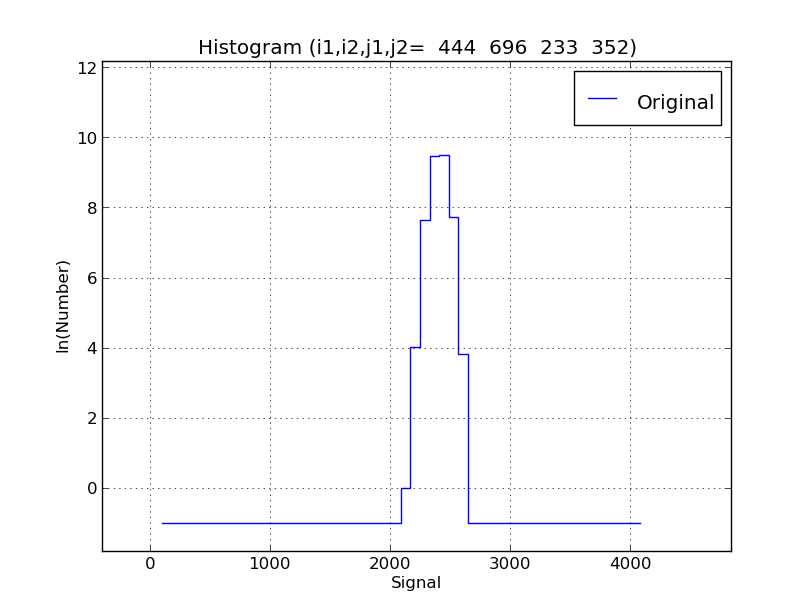 |
An example of making a hitogram plot directly from the List.0 and Axes.0
files that are made by clip_imhist.sh. This has the advantage of making
a simple plot title that tells you the box coordinates for the sub-image
you are histogramming.
% cat Axes.0
Histogram (i1,i2,j1,j2=  444  696  233  352)
   100.00000    4000.00000   Signal
    -1.00000       9.48326   ln(Number)

% cat List.0
clip_imhist.dat      1 2 0 0       line       b - 70     Original

% xyplotter List.0 Axes.0
Note how we make use of the file clip_imhist.dat in making the plot.
|
The second, and more versatile way to plot the hisogram, is to use
xyplotter_auto and the table files made by clip_imhist.sh:
% xyplotter_auto clip_imhist q q 10 N
By specifying the X,Y parameter names as "q" I am queried for them
during the run. Here is the plot I make this way:
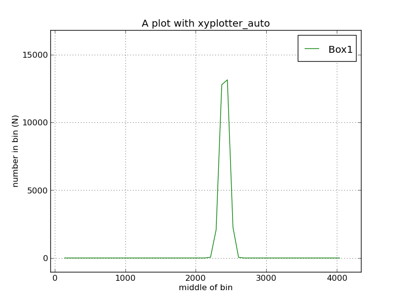 |
An example of making a hitogram plot with the table files and xyplotter_auto.
% xyplotter_auto clip_imhist q q 10 N
Notice that in this example I chose to plot the Number of counts
as oppsed to log(Number). In the first example we are forced to
use log(Number).
|
Back to calling page