 |
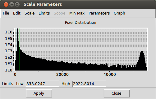
| FIGURE 1: A hstogram of imag pixel values computed with ds9 using the scale option. I can use the mouse to change the green (low, z1) and red (high, z2) lines around. The peak occurs at I=875 in this histogram. |
The cih code computes a histogram of image pixel values. This very simple codes converts every pixel value, P, to an integer: I = P+zadd. Then all integer pixel values, I, are counted for values from 1 to 65536. The user can also generate a file for viewing the histogram with XYP. This is accomplished by setting the values of istart (the first I value to be printed), and nhop (print every nhop pixel value). If istart=0, then no output file (always named "xyp_cih.dat" is generated. As with many BOTW codes, cih is usually run with the script cih.sh:
%  cih.sh o.fits 0.5 10000 3
       0.538       10.286        0.462        0.075        2.849

arg1 - image name (full path)
arg2 - zadd (=0.5 for integer histogram)
arg3 - First value for pixel histogram (XYP) file
arg4 - pixel skip for output (print every arg4-th point)
Usage:  cih.sh o.fit 0.5 5000 4
Note: Use arg3=0 to avoid XYP file dump.

% ls
cih.explain  cih.stndout  S/  t1.fits

% cat cih.explain
# Explanation of cih output (standard out and here)
out1: weighted mean peak value (mean sky)
out2: weighted s.d. of sky
out3: sky peak width at half-power point
out4: z1 (-1 sigma of sky)
out5: z2 (+5 sigma of sky)

% cat cih.stndout
       0.538       10.286        0.462        0.075        2.849
The last three command line arguments deal with creating a file for plotting the histogram. In the example above, because I use arg3=10000, I generate an output file named "xyp_cih.dat". This can be used as input to XYP to view the histogram of the pixels. This XYP file will start with the first bin of the pixel hisogram at I=10000. Every 3rd point (arg4) will be printed. This way, I can see any histogram features out to 66636. This is necessary since XYP plots a maximum of 20000 points.
Notice above that I am now trying to have most OTW scripts write simple data to standard out. At the same time I generate the same output in a file (name_of_code.stndout). I also try to always produce a file (name_of_code.explain) that explains things about the output information.
For the RUN0 case below, I just generate the background information (sent to standard out and the file zrange.from_cih). For the RUN0 case below, I also generate the XYP input file named xyp_cih.dat.
% pwd
/home/sco/sco/projects/Test_Data_for_Codes/T_runs/cih/ex0

% ls
S/

% cat S/RUN0
#!/bin/bash
# Usage:  cih.sh o.fit 0.5 5000 4
cp /home/sco/sco/projects/Test_Data_for_Codes/T_images/S7_magell/n3664_R.fits t1.fits
#
# Run simple
cih.sh t1.fits 0 0 0
#
# Clean up
\rm -f fitsr2048.header_copy header.info  junc runner*

% S/RUN0
       0.538       10.286        0.462        0.075        2.849
% ls
cih.explain  S/  t1.fits  zrange.from_cih

% cat cih.explain
# Explanation of cih output (standard out and here)
arg1: weight mean peak value (mean sky)
arg2: weight s.d. of sky
arg3: sky peak width at half-power point
arg4: z1 (-1 sigma of sky)
arg5: z2 (+5 sigma of sky)

% cat zrange.from_cih
       0.538       10.286        0.462        0.075        2.849


============ I delete everything, and run RUN1

% cat S/RUN1
#!/bin/bash
# Usage:  cih.sh o.fit 0.5 5000 4
cp /home/sco/sco/projects/Test_Data_for_Codes/T_images/S7_magell/n3664_R.fits t1.fits
#
# Run to make XYP file
cih.sh t1.fits 0.0 10  5
#
# Clean up
\rm -f fitsr2048.header_copy header.info  junc runner*

% S/RUN1
       0.538       10.286        0.462        0.075        2.849
% ls
cih.explain  S/  t1.fits  xyp_cih.dat  zrange.from_cih
The ds9 code allows me quick access to the pixel histogram. An example of such a histogram, for the image Rsco5210.fits is shown below. The format of the histogram plot can be changed by selecting the "Current Range" value in graph. Then one can move the red/green lines around and hit the "Apply" button to change the parts of the histogram to be viewed. Using this approach I am able to see that the histogram peak fall at I=875.
|
| FIGURE 1: A hstogram of imag pixel values computed with ds9 using the scale option. I can use the mouse to change the green (low, z1) and red (high, z2) lines around. The peak occurs at I=875 in this histogram. |
I can get a better view of the histogram using cih and the XYP plotting code. To run the cih code, and generate a historgam file for XYP:
cih.sh Rsco5210.fits 0.5 1 4I used XYP to plot the data in the output file called "xyp_cih.dat". With this plot I can clearly see the peak and the 1/2 power position (on the high-side of the peak):
I_peak = 850       y=4.8

At y=2.4 (half power) I find   I = 1035

Hence, the peak widt at half power is about 1035-850 = 185.

If I treat this like a sky sigma, then to plot -1sig to 5sig:
  z1,z2 =  665 , 1775

**** This looks pretty good in a ds9 display!
A useful thing to do is have cih dump values of the PEAK and PEAK_WIDTH (1/2 width really) and then use these values to create better scaled images with ds9 running under ID (Image Display).