As of mid Jun2019 I have reduced 174 acm images through the point of sky surface brightness evaluation. These images are taken from 29 nights in 2018 and 2019. In addition to reducing more nights with a moon at about 50% illumination, some of the new images use the acm B filter. Hence, in this latest data set I have more variation in the data: another filter, different moon conditions, some errant exposure times (EXPTIME .l1. 0.1 sec). In this analysis I want to address the same basic questions having to do with plotting the data:

1. I want to select targets using parameter rules. For instance, I may want to flot g data from times when the moon was down (i.e. PHIMOON=-99.0).
2. I want to always plot from the original table file (A1) and use custom flag files for each new set of points plotted.

 
The images are in:    /home/sco/acm_SBSKY   (see list.05) 
I do analysis in:    /home/sco/scohtm/scocodes/Night_of_acm/Analysis/analysis05_jun13_2019/data   

% ls -1 /home/sco/acm_SBSKY/*fits > list.05 

I make a table file with fits2table. Here is the PARAMS The PARAMS file is 
what determine what will be assembled i the table files.
 
% cat PARAMS
WAVELEN    Filter wavelength (angs) 
UTHOURS    Hours since 0hUT
UTDATE     UT date (YYYYMMDD)
RSTRT      Radius position of tracker at start (mm)
AZHET      HET structure AZ (deg)
MILLUM     percentage moon illumination
PHIMOON    angle of separation to moon (deg)
ZPSEC      ZP for a 1-sec exposure
ZPERR      mean error of ZPSEC
SKYSB      sky surface brightness (mags per sq.arcsec)
SKYSBERR   mean error of SKYSB

To get tables: 
% ACM_ANALYSIS_TABLES list.05 PARAMS N

Make a nice plot: 
% Generic_Points N                        # edit "xyplotter_auto.pars" 

% xyplotter_auto A1 PHIMOON SKYSB 20 N
% xyplotter_auto A1 MILLUM PHIMOON 21 N

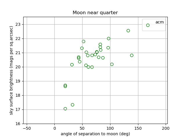
A plot of acm g sky surface brightness (mss) versus the moon separation angle in dgrees. These data were taken from the datg table file produced with a run of ACM_ANALYSIS_TABLES. The dates of images reduced here were chose so that the moon phase was nearly always around 40 to 60 percent illumination. A normalization for moon phase will eventually be made so that the correlation between moon angle and sky surface brightness should tighten up. Here I have used the datb.table file to collect the plotted points.

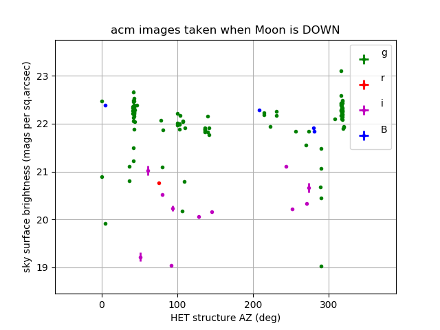
Belwo I use the new table mask tools to plot g,r,i,B sky surface nrightness, taken when the moon is down (PHIMOON=-99).

 
 

xyplotter_auto A1 AZHET SKYSB 30 N 

To make the selections:
% table_text_mask A1 PSYSNAME g mask1                    # select g observations 
% table_fprange_mask A1 PHIMOON -100.0 -90.0  mask2 N    # only points when moon is down 
% masklogic.sh mask1 mask2 and mask3 N                   # make final mask 
% get_table_rows A1 mask3 g_NoMoon                       # Make the final table file of selected data 

Then I simply edit the List.30 file to add this set. 
% xyplotter List.30 Axes.30 N                           # view the full plot 

To do the 4 filters separately: 

% table_fprange_mask A1 PHIMOON -100.0 -90.0 mask2 N     

Collect g data: 
 table_text_mask A1 PSYSNAME g mask1               
 masklogic.sh mask1 mask2 and mask3 N          
 get_table_rows A1 mask3 g_NoMoon             

Collect i data: 
 table_text_mask A1 PSYSNAME i mask1               
 masklogic.sh mask1 mask2 and mask3 N          
 get_table_rows A1 mask3 i_NoMoon             

Collect r data: 
 table_text_mask A1 PSYSNAME r mask1               
 masklogic.sh mask1 mask2 and mask3 N            
 get_table_rows A1 mask3 r_NoMoon               

Collect B data: 
 table_text_mask A1 PSYSNAME B mask1               
 masklogic.sh mask1 mask2 and mask3 N            
 get_table_rows A1 mask3 B_NoMoon               

Make the plot:   xyplotter List.30 Axes.30 N 
 

A plotbrated sky surface brightness in gmrmi,B measure from images taken under moonless and clear conditions. These acm images are taken from 29 nights in 2018 and 2019. The photometrc zeropints were calbrated using PANSTARRS photometry, after WCS calibration was performed with the USNOB-1.0 catalog. No attempt has been made to clean discrepant points. It was discovered that some image with extremely short exposure time still remain in this data set.