I have assembled 71 reduced acm images in /home/sco/acm_SBSKY. These are from 9 nights during the periods around new moon in Feb,Mar,Apr of 2019. I am seeing that during these periods, where we observed primarily hetdex fiedld, the acm images are primarily g filter observations. The few i images seem to be taken outside the 18 degree twilight window.

Here I want to concentrate on building a script that sets up the initial g,i tables. Then I want to make plots and compute stats witj various table/plotter tools in oder to investigate systematics in the g image data.

 
The images are in:     /home/sco/acm_SBSKY   (see list.0) 
I do analysis 02 in:   /home/sco/acm_reds_sco2019/Analyses/Analysis02

% ls -1 /home/sco/acm_SBSKY/*fits > list.02 

I make a table file with fits2table. Here is the PARAMS The PARAMSfile is 
what determine what will be assembled i the table files.
 
% cat PARAMS
WAVELEN    Filter wavelength (angs) 
UTHOURS    Hours since 0hUT
UTDATE     UT date (YYYYMMDD)
RSTRT      Radius position of tracker at start (mm)
AZHET      HET structure AZ (deg)
MILLUM     percentage moon illumination
PHIMOON    angle of separation to moon (deg)
ZPSEC      ZP for a 1-sec exposure
ZPERR      mean error of ZPSEC
SKYSB      sky surface brightness (mags per sq.arcsec)
SKYSBERR   mean error of SKYSB

To get tables: 
% ACM_ANALYSIS_TABLES list.02 PARAMS N

Make a nice plot: 
% Generic_Points N                        # edit "xyplotter_auto.pars" 
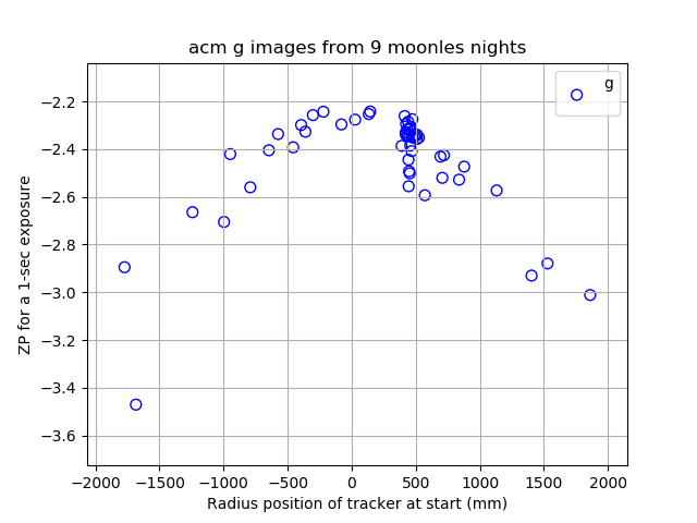
% xyplotter_auto datg RSTRT ZPSEC 20 N        # edir List.20 , Axes.20 hereafter 
% xyplotter_auto dati RSTRT ZPSEC 20 N        # edir List.20 , Axes.20 hereafter 

Using the datg table: 
% point_selector datg RSTRT ZPSEC N

I view (and record) afe bad points. These were: 
/home/sco/acm_SBSKY/20190401T092839.5_acm_sci.fits
/home/sco/acm_SBSKY/20190205T121618.8_acm_sci.fits
/home/sco/acm_SBSKY/20190204T024712.6_acm_sci.fits
/home/sco/acm_SBSKY/20190204T103114.8_acm_sci.fits
/home/sco/acm_SBSKY/20190307T081109.3_acm_sci.fits
/home/sco/acm_SBSKY/20190207T073956.7_acm_sci.fits

I remove these from datg.images to make:   list.02_cleaned_g
Then I make a new datg table: 
% ACM_ANALYSIS_TABLES list.02_cleaned_g PARAMS N
% point_selector datg RSTRT ZPSEC N      # there is a bug here!!!!!

Now I see a clean plot, so I use xyplotter_auto: 
% xyplotter_auto datg RSTRT ZPSEC 10 N 

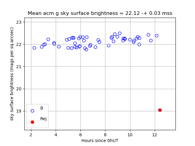
% xyplotter_auto datg UTHOURS SKYSB 20 N 
*** I see one bad poin
% point_selector datg UTHOURS SKYSB N       # mark the bad point
% point_selector_stats.sh xyf.in Y 0 N  
    22.12446     22.16460      0.19432      0.02669       53   (mean,mediam,sig,me,n)
Hence, excluding the one bad point taken after 12h UT the mean 
g sky surface brightness is   22.12 -+ 0.03 

I put thsi in the Axes.20 file and replot with:
% xyplotter List.20 Axes.20 N  


 

The ZPSEC (ZP for a 1-sec image) plotted as a function of the distance from tracker center (in mm). All photometric ZP solutions were obtained vis cross-match to PANSTARRS (gri) using stars only. The points are from acm g images collected from 9 nights very close to new moon. The current Y axis values are in magnitude units, but these data can be used to evaluate the observed HET illumination function.

Using the points from the previous Figure I plot the g sky surface brightness in units of magnitudes per square arcsec) from 54 images taken on 9 different nights close to new moon. The red point was taken after 18deg twilight and was rejected from computing a mean value of Mean sky surface brightbness (g) = 22.12 -+ 0.03 mss I use the UT time in hours on the X axis to show approximately at what point in the night each image was taken. There is some evidence that the sky darkens systematically through the night. For comparison, the mean CTIO g sky surface brightness is recorded as 22.3 mss. Hence, McDonald is slighly brighter in the mean.